2.2: Best Affine Approximations

In this section we will generalize the basic ideas of the differential calculus of functions \(f: \mathbb{R} \rightarrow \mathbb{R}\) to functions \(f: \mathbb{R} \rightarrow \mathbb{R}^{n}\). Recall that given a function \(f: \mathbb{R} \rightarrow \mathbb{R}\), we say \(f\) is differentiable at a point \(c\) if there exists an affine function \(A: \mathbb{R} \rightarrow \mathbb{R}\), \(A(x)=m(x-c)+f(c)\), such that

\[ \lim _{h \rightarrow 0} \frac{f(c+h)-A(c+h)}{h}=0 . \label{2.2.1} \]

We call \(A\) the best affine approximation to \(f\) at \(c\) and \(m\) the derivative of \(f\) at \(c\), denoted \(f^{\prime}(c)\). Moreover, we call the the graph of \(A\), that is, the line with equation

\[ y=f^{\prime}(c)(x-c)+f(c),\]

the tangent line to the graph of \(f\) at \((c, f(c))\).

The condition (\(\ref{2.2.1}\)) says that the function \(\varphi(h)=f(c+h)-A(c+h) \text { is } o(h)\). In general, we say a function \(\varphi: \mathbb{R} \rightarrow \mathbb{R}\) is \(o(h)\) if

\[ \lim _{h \rightarrow 0} \frac{\varphi(h)}{h}=0 .\]

Best affine approximations

Generalizing the idea of the best affine approximation to the case of a function \(f: \mathbb{R} \rightarrow \mathbb{R}^{n}\) requires only a slight modification of the requirement that \(f(c+h)-A(c+h)\) be \(o(h)\). Namely, since \(f(c+h)-A(c+h)\) is a vector in \(\mathbb{R}^{n}\), we will require that \(\|f(c+h)-A(c+h)\|\), instead of \(f(c+h)-A(c+h)\), be \(o(h)\). If \(n=1\), this will reduce to the one-variable definition since, in that case, \(\|f(c+h)-A(c+h)\|=|f(c+h)-A(c+h)|\) and a function \(\varphi: \mathbb{R} \rightarrow \mathbb{R}\) is \(o(h)\) if and only if \(|\varphi(h)|\) is \(o(h)\).

Definition \(\PageIndex{1}\)

Suppose \(f: \mathbb{R} \rightarrow \mathbb{R}^{n}\) and \(c\) is a point in the domain of \(f\). We call an affine function \(A: \mathbb{R} \rightarrow \mathbb{R}^{n}\) the best affine approximation to \(f\) at \(c\) if (1) \(A(c)=f(c)\) and (2) \(\|R(h)\|\) is \(o(h)\), where

\[ R(h)=f(c+h)-A(c+h). \]

Suppose \(f: \mathbb{R} \rightarrow \mathbb{R}^{n}\) and \(A: \mathbb{R} \rightarrow \mathbb{R}^{n}\) is an affine function for which \(A(c)=f(c)\). Since \(A\) is affine, there exists a linear function \(L: \mathbb{R} \rightarrow \mathbb{R}^{n}\) and a vector \(\mathbf{b}\) in \(\mathbb{R}^n\) such that \(A(t)=L(t)+\mathbf{b}\) for all \(t\) in \(\mathbb{R}\). Since we have

\[ f(c)=A(c)=L(c)+\mathbf{b},\]

it follows that \(\mathbf{b}=f(c)-L(c)\). Hence for all \(t\) in \(\mathbb{R}\),

\[A(t)=L(t)+f(c)-L(c)=L(c-t)+f(c).\]

Moreover, if \(\mathbf{a}=L(1)\), then, from our results in Section 1.5,

\[ A(t)=\mathbf{a}(t-c)+f(c).\]

Hence

\[ R(h)=f(c+h)-A(c+h)=f(c+h)-f(c)-\mathbf{a} h , \]

from which it follows that

\[\begin{align}
\lim _{h \rightarrow 0^{+}} \frac{\|R(h)\|}{h} &=\lim _{h \rightarrow 0^{+}} \frac{\|f(c+h)-f(c)-\mathbf{a} h\|}{h} \nonumber \\
&=\lim _{h \rightarrow 0^{+}}\left\|\frac{f(c+h)-f(c)-\mathbf{a} h}{h}\right\| \label{} \\
&=\lim _{h \rightarrow 0^{+}}\left\|\frac{f(c+h)-f(c)}{h}-\mathbf{a}\right\| \nonumber
\end{align} \]

Thus

\[ \lim _{h \rightarrow 0^{+}} \frac{\|R(h)\|}{h}=0 \nonumber \]

if and only if

\[ \lim _{h \rightarrow 0^{+}} \frac{f(c+h)-f(c)}{h}=\mathbf{a}. \nonumber \]

A similar calculation from the left shows that

\[\lim _{h \rightarrow 0^{-}} \frac{\|R(h)\|}{h}=0 \nonumber \]

if and only if

\[ \lim _{h \rightarrow 0^{-}} \frac{f(c+h)-f(c)}{h}=\mathbf{a}.\nonumber \]

Hence

\[ \lim _{h \rightarrow 0} \frac{\|R(h)\|}{h}=0\]

if and only if

\[ \lim _{h \rightarrow 0} \frac{f(c+h)-f(c)}{h}=\mathbf{a}.\]

That is, \(A\) is the best affine approximation to \(f\) at \(c\) if and only if, for all \(t\) in \(\mathbb{R}\),

\[ A(t)=\mathbf{a}(t-c)+f(c), \]

where

\[ \mathbf{a}=\lim _{h \rightarrow 0} \frac{f(c+h)-f(c)}{h}.\]

Definition \(\PageIndex{2}\)

Suppose \(f: \mathbb{R} \rightarrow \mathbb{R}^{n}\). If

\[ \lim _{h \rightarrow 0} \frac{f(c+h)-f(c)}{h}\]

exists, then we say \(f\) is differentiable at \(c\) and we call

\[ D f(c)=\lim _{h \rightarrow 0} \frac{f(c+h)-f(c)}{h} \label{2.2.15} \]

the derivative of \(f\) at \(c\).

Note that (\(\ref{2.2.15}\)) is the same as the formula for the derivative in one-variable calculus. In fact, in the case \(n=1\), (\(\ref{2.2.15}\)) is just the derivative from one-variable calculus. However, if \(n>1\), then \(D f(c)\) will be a vector, not a scalar.

The following theorem summarizes our work above.

Theorem \(\PageIndex{1}\)

Suppose \(f: \mathbb{R} \rightarrow \mathbb{R}^{n}\) and \(c\) is a point in the domain of \(f\). Then \(f\) has a best affine approximation \(A: \mathbb{R} \rightarrow \mathbb{R}^{n}\) at \(c\) if and only if \(f\) is differentiable at \(c\), in which case

\[ A(t)=D f(c)(t-c)+f(c) .\]

We saw in Section 2.1 that a limit of a vector-valued function \(f\) may be computed by evaluating the limit of each coordinate function separately. This result has an important consequence for computing derivatives. Suppose \(f: \mathbb{R} \rightarrow \mathbb{R}^{n}\) is differentiable at \(c\). If we write

\[ f(t)=\left(f_{1}(t), f_{2}(t), \ldots, f_{n}(t)\right. , \nonumber \]

then

\[ \begin{aligned}
D f(c) &=\lim _{h \rightarrow 0} \frac{f(c+h)-f(c)}{h} \\
&=\lim _{h \rightarrow 0} \frac{1}{h}\left(\left(f_{1}(c+h), f_{2}(c+h), \ldots, f_{n}(c+h)-\left(f_{1}(c), f_{2}(c), \ldots, f_{n}(c)\right)\right.\right.\\
&=\lim _{h \rightarrow 0}\left(\frac{f_{1}(c+h)-f_{1}(c)}{h}, \frac{f_{2}(c+h)-f_{2}(c)}{h}, \ldots, \frac{f_{n}(c+h)-f_{n}(c)}{h}\right) \\
&=\left(\lim _{h \rightarrow 0} \frac{f_{1}(c+h)-f_{1}(c)}{h}, \lim _{h \rightarrow 0} \frac{f_{2}(c+h)-f_{2}(c)}{h}, \ldots, \lim _{h \rightarrow 0} \frac{f_{n}(c+h)-f_{n}(c)}{h}\right) \\
&=\left(f_{1}^{\prime}(c), f_{2}^{\prime}(c), \ldots, f_{n}^{\prime}(c)\right) .
\end{aligned} \]

In words, the derivative of \(f\) is the vector whose coordinates are the derivatives of the coordinate functions of \(f\), reducing the problem of differentiating vector-valued functions to the problem of differentiation in single-variable calculus.

Proposition \(\PageIndex{1}\)

If \(f\) is differentiable at \(c\) and \(f(t)=\left(f_{1}(t), f_{2}(t), \ldots, f_{n}\left(t_{0}\right)\right)\), then each coordinate function \(f_{k}, k=1,2, \ldots, n\), is differentiable at \(c\) and

\[ D f(c)=\left(f_{1}^{\prime}(c), f_{2}^{\prime}(c), \ldots, f_{n}^{\prime}(c)\right) .\]

For an arbitrary point \(t\) at which \(f\) is differentiable, we will write,

\[ D f(t)=\lim _{h \rightarrow 0} \frac{f(t+h)-f(t)}{h}=\left(f_{1}^{\prime}(t), f_{2}^{\prime}(t), \ldots, f_{n}^{\prime}(t)\right) .\]

That is, we may think of \(Df\) as a vector-valued function itself, with domain being the set of points at which \(f\) is differentiable.

Now suppose \(f: \mathbb{R} \rightarrow \mathbb{R}^{n}\) parametrizes a curve \(C\) and is differentiable at \(c\). If \(D f(c) \neq \mathbf{0}\), then the best affine approximation

\[ A(t)=D f(c)(t-c)+f(c) \nonumber \]

parametrizes a line, a line which best approximates the curve \(C\) for points near \(f(c)\). On the other hand, if \(D f(c)=\mathbf{0}\), then \(A\) is a constant function with range consisting of the single point \(f(c)\). These considerations motivate, in part, the following definitions.

Definition \(\PageIndex{3}\)

Suppose \(f: \mathbb{R} \rightarrow \mathbb{R}^{n}\) is differentiable on \((a,b)\) and \(\mathbf{x}=f(t)\) is a parametrization of a curve \(C\) for \(a<t<b\). If \(D f(t)\) is continuous and \(D f(t) \neq \mathbf{0}\) for all \(t\) in \((a,b)\), then we call \(f\) a smooth parametrization of \(C\).

Definition \(\PageIndex{4}\)

Suppose \(f: \mathbb{R} \rightarrow \mathbb{R}^{n}\) parametrizes a curve \(C\) in \(\mathbb{R}^{n}\) and let \(A\) be the best affine approximation to \(f\) at \(c\). If \(f\) is smooth on some open interval containing \(c\), then we call the line in \(\mathbb{R}^{n}\) parametrized by \(A\) the tangent line to \(C\) at \(f(c)\).

Example \(\PageIndex{1}\)

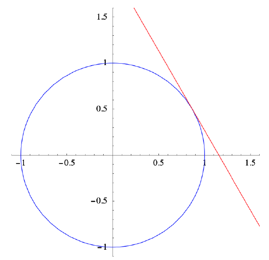
Define \(f: \mathbb{R} \rightarrow \mathbb{R}^{n}\) by \(f(t)=(\cos (t), \sin (t))\) for \(-\infty<t<\infty\). Then, as we saw in Section 2.1, \(f\) parametrizes the unit circle \(C\) centered at the origin. Now

\[ D f(t)=(-\sin (t), \cos (t)), \nonumber \]

so \(Df(t)\) is continuous and \(\|D f(t)\|=1\) for all \(t\). Thus \(f\) is a smooth parametrization of \(C\). For example,

\[ D f\left(\frac{\pi}{6}\right)=\left(-\frac{1}{2}, \frac{\sqrt{3}}{2}\right) \nonumber \]

and

\[ f\left(\frac{\pi}{6}\right)=\left(\frac{\sqrt{3}}{2}, \frac{1}{2}\right) , \nonumber \]

so the best affine approximation to \(f\) at \(t=\frac{\pi}{6}\) is

\[ A(t)=\left(-\frac{1}{2}, \frac{\sqrt{3}}{2}\right)\left(t-\frac{\pi}{6}\right)+\left(\frac{\sqrt{3}}{2}, \frac{1}{2}\right) . \nonumber \]

Figure 2.2.1 shows \(C\) along with the tangent line to \(C\) at \(t=\frac{\pi}{6}\)

Figure \(\PageIndex{1}\): Unit circle with tangent line at \(\left(\frac{\sqrt{3}}{2}, \frac{1}{2}\right)\)

Example \(\PageIndex{2}\)

Suppose we define \(g: \mathbb{R} \rightarrow \mathbb{R}^{2}\) by \(g(t)=(\sin (2 \pi t), \cos (2 \pi t))\), \(-\infty<t<\infty\). Then, as we saw in Section 2.1, \(g\) parametrizes the same circle \(C\) as \(f\) in the previous example. Moreover,

\[ D g(t)=(2 \pi \cos (2 \pi t),-2 \pi \sin (2 \pi t)) \nonumber \]

and \(\|D g(t)\|=1\) for all \(t\), so \(g\) is a smooth parametrization of \(C\). However,

\[ g\left(\frac{1}{6}\right)=\left(\frac{\sqrt{3}}{2}, \frac{1}{2}\right)=f\left(\frac{\pi}{6}\right) ; \nonumber \]

that is, \(g(t)\) is at \(\left(\frac{\sqrt{3}}{2}, \frac{1}{2}\right)\) when \(t=\frac{1}{6}\), whereas \(f(t)\) is at \(\left(\frac{\sqrt{3}}{2}, \frac{1}{2}\right)\) when \(t=\frac{\pi}{6}\). Moreover,

\[ D g\left(\frac{1}{6}\right)=(\pi,-\pi \sqrt{3}), \nonumber \]

so the best affine approximation to \(g\) at \(t=\frac{1}{6}\) is

\[ B(t)=(\pi,-\pi \sqrt{3})\left(t-\frac{1}{6}\right)+\left(\frac{\sqrt{3}}{2}, \frac{1}{2}\right) . \nonumber \]

Note that although \(A\), the best affine approximation to \(f\) at \(t=\frac{1}{6}\), and \(B\), the best affine approximation to \(g\) at \(t=\frac{1}{6}\), are different functions, they parametrize the same line since

\[ (\pi,-\pi \sqrt{3})=-2 \pi\left(-\frac{1}{2}, \frac{\sqrt{3}}{2}\right) .\nonumber \]

Example \(\PageIndex{3}\)

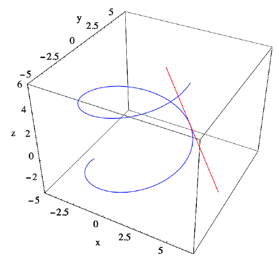
Consider the helix \(C\) parametrized by \(f: \mathbb{R} \rightarrow \mathbb{R}^{3}\) defined by

\[ f(t)=(4 \cos (t), 4 \sin (t), t) . \nonumber \]

Then

\[ D f(t)=(-4 \sin (t), 4 \cos (t), 1) .\nonumber \]

Since \(Df\) is continuous and

\[ \|D f(t)\|=\sqrt{16 \sin ^{2}(t)+16 \cos ^{2}(t)+1}=\sqrt{17} \nonumber \]

for all \(t\), \(f\) is a smooth parametrization of \(C\). Now, for example,

\[ D f\left(\frac{\pi}{4}\right)=\left(-\frac{4}{\sqrt{2}}, \frac{4}{\sqrt{2}}, 1\right)=(-2 \sqrt{2}, 2 \sqrt{2}, 1) \nonumber \]

and

\[ f\left(\frac{\pi}{4}\right)=\left(\frac{4}{\sqrt{2}}, \frac{4}{\sqrt{2}}, \frac{\pi}{4}\right)=\left(2 \sqrt{2}, 2 \sqrt{2}, \frac{\pi}{4}\right),\nonumber \]

so the best affine approximation to \(f\) at \(t=\frac{\pi}{4}\) is

\[ A(t)=(-2 \sqrt{2}, 2 \sqrt{2}, 1)\left(t-\frac{\pi}{4}\right)+\left(2 \sqrt{2}, 2 \sqrt{2}, \frac{\pi}{4}\right) .\nonumber \]

The helix \(C\) and the line parametrized by \(A\), namely, the tangent line to \(C\) at \(t=\frac{\pi}{4}\), are shown in Figure 2.2.2.

Figure \(\PageIndex{2}\): Helix with tangent line at \(\left(2 \sqrt{2}, 2 \sqrt{2}, \frac{\pi}{4}\right)\)

Example \(\PageIndex{4}\)

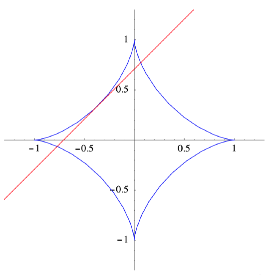
Let \(C\) be the curve in \(\mathbb{R}^2\) parametrized by

\[ h(t)=\left(\cos ^{3}(t), \sin ^{3}(t)\right) . \nonumber \]

Then

\[ D h(t)=\left(-3 \cos ^{2}(t) \sin (t), 3 \sin ^{2}(t) \cos (t)\right) . \nonumber \]

Hence \(Dh\) is continuous for all \(t\), but \(h\) is not a smooth parametrization of \(C\) since \(D h(t)=\mathbf{0}\) whenever \(t\) is an integer multiple of \(\frac{pi}{2}\). These points correspond to the sharp corners of \(C\) at (1,0), (0,1), (−1,0, and (0,−1), as shown in Figure 2.2.3. However, \(h\) is a smooth parametrization of the four arcs of \(C\) which are parametrized by restricting \(h\) to the open intervals \(\left(0, \frac{\pi}{2}\right),\left(\frac{\pi}{2}, \pi\right),\left(\pi, \frac{3 \pi}{2}\right)\), and \(\left(\frac{3 \pi}{2}, 2 \pi\right)\). Hence, for example, noting that

\[ D h\left(\frac{3 \pi}{4}\right)=\left(-\frac{3}{2 \sqrt{2}},-\frac{3}{2 \sqrt{2}}\right) \nonumber \]

and

\[ h\left(\frac{3 \pi}{4}\right)=\left(-\frac{1}{2 \sqrt{2}}, \frac{1}{2 \sqrt{2}}\right) ,\nonumber \]

we find that the best affine approximation to \(h\) at \(t=\frac{3 \pi}{4}\) is

\[ A(t)=\left(-\frac{3}{2 \sqrt{2}},-\frac{3}{2 \sqrt{2}}\right)\left(t-\frac{3 \pi}{4}\right)+\left(-\frac{1}{2 \sqrt{2}}, \frac{1}{2 \sqrt{2}}\right) .\nonumber \]

The tangent line parametrized by \(A\) is shown in Figure 2.2.3.

Figure \(\PageIndex{3}\): \(h(t)=\left(\cos ^{3}(t), \sin ^{3}(t)\right)\) with tangent line at \(\left(-\frac{1}{2 \sqrt{2}}, \frac{1}{2 \sqrt{2}}\right)\)

Proposition \(\PageIndex{2}\)

Suppose \(f: \mathbb{R} \rightarrow \mathbb{R}^{n}\), \(g: \mathbb{R} \rightarrow \mathbb{R}^{n}\), and \(\varphi: \mathbb{R} \rightarrow \mathbb{R}\) are all differentiable. Then

\[ \begin{align}
D(f(t)+g(t))=D f(t)+D g(t), \label{2.2.19} \\
D(f(t)-g(t))=D f(t)-D g(t), \label{2.2.20} \\
D(\varphi(t) f(t))=\varphi(t) D f(t)+\varphi^{\prime}(t) f(t), \label{2.2.21} \\
\frac{d}{d t}(f(t) \cdot g(t))=f(t) \cdot D g(t)+D f(t) \cdot g(t), \label{2.2.22}
\end{align} \]

and

\[ D\left(f(\varphi(t))=D f(\varphi(t)) \varphi^{\prime}(t)\right) . \label{2.2.23}\]

Note that all of the statements in this proposition reduce to familiar results from one-variable calculus when \(n=1\). To verify these results, let

\[ f(t)=\left(f_{1}(t), f_{2}(t), \ldots, f_{n}(t)\right) \nonumber \]

and

\[ g(t)=\left(g_{1}(t), g_{2}(t), \ldots, g_{n}(t)\right) .\nonumber \]

Then

\[ \begin{align}
D(f(t)+g(t)) &=D\left(f_{1}(t)+g_{1}(t), f_{2}(t)+g_{2}(t), \ldots, f_{n}(t)+g_{n}(t)\right) \nonumber \\
&=\left(f_{1}^{\prime}(t)+g_{1}^{\prime}(t), f_{2}^{\prime}(t)+g_{2}^{\prime}(t), \ldots, f_{n}^{\prime}(t)+g_{n}^{\prime}(t)\right) \label{} \\
&=\left(f_{1}^{\prime}(t), f_{2}^{\prime}(t), \ldots, f_{n}^{\prime}(t)\right)+\left(g_{1}^{\prime}(t), g_{2}^{\prime}(t), \ldots, g_{n}^{\prime}(t)\right) \nonumber \\
&=D f(t)+D g(t), \nonumber
\end{align} \]

verifying (\(\ref{2.2.19}\)). The verification of (2.1.20) is similar. The demonstrations of (\(\ref{2.2.21}\)) and (2.1.22), both of which are generalizations of the product rule from one-variable calculus, follow easily from that result; we will check (2.1.22) here and leave (\(\ref{2.2.21}\)) for Exercise 13. Using the product rule, we have

\[ \begin{align}
\frac{d}{d t}(f(t) \cdot g(t))=& \frac{d}{d t}\left(f_{1}(t) g_{1}(t)+f_{2}(t) g_{2}(t)+\cdots+f_{n}(t) g_{n}(t)\right) \nonumber \\
=& f_{1}(t) g_{1}^{\prime}(t)+f_{1}^{\prime}(t) g_{1}(t)+f_{2}(t) g_{2}^{\prime}(t)+f_{2}^{\prime}(t) g_{2}(t)+\cdots \label{} \\
& \quad+f_{n}(t) g_{n}^{\prime}(t)+f_{n}^{\prime}(t) g_{n}(t) \nonumber \\
=& f(t) \cdot D g(t)+D f(t) \cdot g(t). \nonumber
\end{align} \]

Finally, (\(\ref{2.2.23}\)), a generalization of the chain rule from one-variable calculus, follows directly from that result:

\[ \begin{align}
D(f(\varphi(t))) &=D\left(f_{1}(\varphi(t)), f_{2}(\varphi(t)), \ldots, f_{n}(\varphi(t))\right) \nonumber \\
&=\left(f_{1}^{\prime}(\varphi(t)) \varphi^{\prime}(t), f_{2}^{\prime}(\varphi(t)) \varphi^{\prime}(t), \ldots, f_{n}^{\prime}(\varphi(t)) \varphi^{\prime}(t)\right) \label{} \\
&=D f(\varphi(t)) \varphi^{\prime}(t). \nonumber
\end{align} \]

Reparametrizations

We have seen above that the parametrization of a curve \(C\) in \(\mathbb{R}^n\) is not unique. For example, we saw that both \(f(t)=(\cos (t), \sin (t))\) and \(g(t)=(\sin (2 \pi t), \cos (2 \pi t))\) parametrize the unit circle centered at the origin. However, we also noted that the best affine approximations for the two parametrizations, although distinct functions, nevertheless parametrize the same line at \(\left(\frac{\sqrt{3}}{2}, \frac{1}{2}\right)\), the line we have been calling the tangent line. We should suspect that this will be the case in general, that is, the tangent line to a curve \(C\) at a particular point should not depend on the particular parametrization of \(C\) used in the computation. While avoiding some technicalities, we will provide some justification for these ideas.

Definition \(\PageIndex{5}\)

Suppose \(\mathbf{x}=f(t), a<t<b\), is a smooth parametrization of a curve \(C\) in \(\mathbb{R}^n\). Suppose \(\varphi: \mathbb{R} \rightarrow \mathbb{R}\) has domain \((c,d)\), range \((a,b)\), and \(\varphi^{\prime}\) exists and is continuous on \((c,d)\). If \(\varphi^{\prime}(t) \neq 0\) for all \(t\) in \((c,d)\), then we call \(g(t)=f(\varphi(t))\) a reparametrization of \(f\).

Example \(\PageIndex{5}\)

Let \(f(t)=(\cos (t), \sin (t))\) and \(g(t)=(\sin (2 \pi t), \cos (2 \pi t))\). Since

\[ \sin (t)=\cos \left(\frac{\pi}{2}-t\right) \nonumber \]

and

\[\cos (t)=\sin \left(\frac{\pi}{2}-t\right), \nonumber \]

it follows that

\[ g(t)=f\left(\frac{\pi}{2}-2 \pi t\right)=f(\varphi(t)), \nonumber \]

where

\[ \varphi(t)=\frac{\pi}{2}-2 \pi t . \nonumber \]

That is, \(g\) is a reparametrization of \(f\).

Now if \(\mathbf{x}=f(t), a<t<b\), is a smooth parametrization of a curve \(C\) in \(\mathbb{R}^n\) and \(g(t)=f(\varphi(t)), c<t<d\), is a reparametrization of \(f\), then for any \(\alpha\) in \((c,d)\),

\[ D g(\alpha)=D\left(f(\varphi(\alpha))=D f(\varphi(\alpha)) \varphi^{\prime}(\alpha)\right. . \]

Hence \(Dg(\alpha)\) and \(D f(\varphi(\alpha))\) are parallel, the former being the latter multiplied by the scalar \(\varphi^{\prime}(\alpha)\). In other words, the lines parametrized by the best affine approximation to \(g\) at \(t=\alpha\) and the best affine approximation to \(f\) at \(t=\varphi(\alpha)\) are the same.

Example \(\PageIndex{6}\)

In our previous example, we have

\[ \varphi^{\prime}(t)=-2 \pi , \nonumber \]

so, for any \(\alpha\), we should have

\[ D g(\alpha)=-2 \pi D f(\varphi(\alpha)). \nonumber \]

This agrees with our previous calculation using \(\alpha=\frac{1}{6}\).

Tangent and normal vectors

If \(f: \mathbb{R} \rightarrow \mathbb{R}^{n}\) is a smooth parametrization of a curve \(C\), then, for any \(t\), \(Df(t)\) is the direction of the tangent line to \(C\) at \(f(t)\). Moreover, from our discussion above, if \(g\) is a reparametrization of \(f\), say, \(g(t)=f(\varphi(t))\), then \(Dg(t)\) and \(D f(\varphi(t))\) will have the same or opposite direction. In other words, the direction of the tangent line either remains the same or is reversed under reparametrization. On the other hand,

\[ \|D g(t)\|=\|D f(\varphi(t))\|\left|\varphi^{\prime}(t)\right| .\]

As we should expect, although both \(Dg(t)\) and \(D f(\varphi(T))\) are tangent to the curve at \(g(t)\), their lengths do not have to be the same. In Section 2.3 we will discuss how we may think of this in terms of the speed of a particle moving along the curve \(C\), with its position on \(C\) at time t given by either \(g(t)\) or \(f(t)\).

For these and other considerations, it is useful to define a standard tangent vector, unique up to a change in sign.

Definition \(\PageIndex{6}\)

If \(f: \mathbb{R} \rightarrow \mathbb{R}^{n}\) is a smooth parametrization of a curve \(C\), then we call

\[ T(t)=\frac{D f(t)}{\|D f(t)\|} \]

the unit tangent vector to \(C\) at \(f(t)\).

From the preceding, we must keep in mind that the unit tangent vector \(T(t)\) is always in reference to some parametrization \(f\) of the curve \(C\). Essentially, this is a choice of an orientation for the curve, that is, the direction of motion for a particle whose position at time \(t\) is given by \(f(t)\).

If \(\mathbf{x}=f(t), a<t<b\), is a smooth parametrization of a curve \(C\) in \(\mathbb{R}^n\), then, by definition, \(\|T(t)\|=1\) for all \(t\) in \((a,b)\). Hence

\[ T(t) \cdot T(t)=1 \label{2.2.30} \]

for all \(t\) in \((a,b)\). Differentiating (\(\ref{2.2.30}\)), we have

\[ \frac{d}{d t}(T(t) \cdot T(t))=\frac{d}{d t} 1=0 ,\]

and so, using (\(\ref{2.2.22}\)), we have

\[ 0=\frac{d}{d t}(T(t) \cdot T(t))=T(t) \cdot D T(t)+D T(t) \cdot T(t)=2 D T(t) \cdot T(t) \]

for all \(t\) in \((a,b)\). Thus \(T(t) \cdot D T(t)=0\) for \(a<t<b\). In other words, \(DT(t)\) is orthogonal to \(T(t)\) for all \(t\) in \((a,b)\).

Definition \(\PageIndex{7}\)

If \(f: \mathbb{R} \rightarrow \mathbb{R}^{n}\) is a smooth parametrization of a curve \(C\), \(T(t)\) is the unit tangent vector to \(C\) at \(f(t)\), and \(D T(t) \neq \mathbf{0}\), then we call

\[ N(t)=\frac{D T(t)}{\|D T(t)\|} \]

the principal unit normal vector to \(C\) at \(f(t)\).

Example \(\PageIndex{7}\)

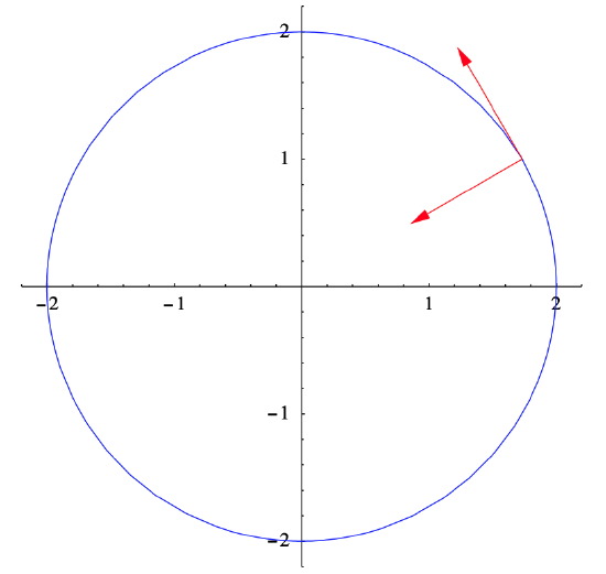
Consider the parametrization of the circle in \(\mathbb{R}^2\) with radius 2 and center at the origin given by

\[ f(t)=(2 \cos (4 t), 2 \sin (4 t)) . \nonumber \]

Then

\[ D f(t)=(-8 \sin (4 t), 8 \cos (4 t)) \nonumber \]

and

\[ \|D f(t)\|=\sqrt{64 \sin ^{2}(4 t)+64 \cos ^{2}(4 t)}=8 . \nonumber \]

Thus the unit tangent vector is

\[ T(t)=\frac{D f(t)}{\|D f(t)\|}=(-\sin (4 t), \cos (4 t)) . \nonumber \]

Moreover,

\[ D T(t)=(-4 \cos (t),-4 \sin (4 t)) , \nonumber \]

so

\[ \|D T(t)\|=\sqrt{16 \cos ^{2}(4 t)+16 \sin ^{2}(4)}=4 , \nonumber \]

and the principal unit normal vector is

\[ N(t)=\frac{D T(t)}{\|D T(t)\|}=(-\cos (4 t),-\sin (4 t)) . \nonumber \]

For example, when \(t=\frac{\pi}{24}\) we have

\[ \begin{gathered}
f\left(\frac{\pi}{24}\right)=(\sqrt{3}, 1), \\
T\left(\frac{\pi}{24}\right)=\left(-\frac{1}{2}, \frac{\sqrt{3}}{2}\right) ,
\end{gathered}\]

and

\[ N\left(\frac{\pi}{24}\right)=\left(-\frac{\sqrt{3}}{2},-\frac{1}{2}\right) .\nonumber \]

Note that, for any value of \(t\), \(f(t) \perp T(t), T(t) \perp N(t)\) (as is always the case), and \(N(t)=-\frac{1}{2} f(t)\)). See Figure 2.2.4.

Figure \(\PageIndex{4}\): A circle with unit tangent and normal vectors

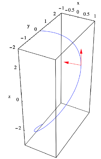
Example \(\PageIndex{8}\)

Consider the elliptical helix \(H\) parametrized by

\[ g(t)=(\cos (t), 2 \sin (t), t) . \nonumber \]

Then

\[ D g(t)=(-\sin (t), 2 \cos (t), 1), \nonumber \]

so

\[ \begin{aligned}
\|D g(t)\| &=\sqrt{\sin ^{2}(t)+4 \cos ^{2}(t)+1} \\
&=\sqrt{\sin ^{2}(t)+\cos ^{2}(t)+3 \cos ^{2}(t)+1} \\
&=\sqrt{2+3 \cos ^{2}(t)} \\
&=\sqrt{2+\frac{3}{2}(1+\cos (2 t))} \\
&=\sqrt{\frac{7+3 \cos (2 t)}{2}} .
\end{aligned}\]

Hence the unit tangent vector is

\[ T(t)=\sqrt{\frac{2}{7+3 \cos (2 t)}}(-\sin (t), 2 \cos (t), 1) . \nonumber \]

Differentiating using (\(\ref{2.2.21}\)), we have

\[ \begin{aligned}
D T(t)=& \sqrt{\frac{2}{7+3 \cos (2 t)}}(-\cos (t),-2 \sin (t), 0) \\
&+\frac{1}{2}\left(\frac{2}{7+3 \cos (2 t)}\right)^{-\frac{1}{2}}\left(\frac{12 \sin (2 t)}{(7+3 \cos (2 t))^{2}}\right)(-\sin (t), 2 \cos (t), 1) \\
=& \sqrt{\frac{2}{7+3 \cos (2 t)}}(-\cos (t),-2 \sin (t), 0)+\frac{3 \sqrt{2} \sin (2 t)}{(7+3 \cos (2 t))^{\frac{3}{2}}}(-\sin (t), 2 \cos (t), 1) .
\end{aligned}\]

For example, at \(t=\frac{\pi}{4}\) we have

\[ \begin{aligned}
g\left(\frac{\pi}{4}\right) &=\left(\frac{1}{\sqrt{2}}, \sqrt{2}, \frac{\pi}{4}\right) , \\
T\left(\frac{\pi}{4}\right) &=\frac{1}{\sqrt{7}}(-1,2, \sqrt{2}) ,
\end{aligned}\]

and

\[ D T\left(\frac{\pi}{4}\right)=\frac{1}{\sqrt{7}}(-1,-2,0)+\frac{3}{7^{\frac{3}{2}}}(-1,2, \sqrt{2})=\frac{1}{7 \sqrt{7}}(-10,-8,3 \sqrt{2}) . \nonumber \]

Thus

\[ \left\|D T\left(\frac{\pi}{4}\right)\right\|=\frac{1}{7 \sqrt{7}} \sqrt{100+64+18}=\frac{\sqrt{26}}{7} , \nonumber \]

so the principal unit normal vector at \(t=\frac{\pi}{4}\) is

\[ N\left(\frac{\pi}{4}\right)=\frac{D T\left(\frac{\pi}{4}\right)}{\left\|D T\left(\frac{\pi}{4}\right)\right\|}=\frac{1}{\sqrt{182}}(-10,-8,3 \sqrt{2}) . \nonumber \]

See Figure 2.2.5

Figure \(\PageIndex{5}\): An elliptical helix with unit tangent and normal vectors

As the last example shows, the computations involved in finding the unit tangent vector and the principal unit normal vector can become involved. In fact, that is why we computed the principal unit normal vector only in the particular case \(t=\frac{\pi}{4}\) instead of writing out the general formula for \(N(t)\). In general these computations can become involved enough that it is often wise to make use of a computer algebra system.