3.5: Extreme Values

After a few preliminary results and definitions, we will apply our work from the previous sections to the problem of finding maximum and minimum values of scalar-valued functions of several variables. The story here parallels to a great extent the story from one-variable calculus, with the inevitable twists and turns due to the presence of additional variables. We will begin with a definition very similar to the analogous definition for functions of a single variable.

The Extreme Value Theorem

Definition \(\PageIndex{1}\)

Suppose \(f: \mathbb{R}^{n} \rightarrow \mathbb{R}\) is defined on a set \(S\). We say \(f\) has a maximum value of \(M\) at \(\mathbf{c}\) if \(f(\mathbf{c})=M\) and \(M \geq f(\mathbf{x})\) for all \(\mathbf{x}\) in \(S\). We say \(f\) has a minimum value of \(m\) at \(\mathbf{c}\) if \(f(\mathbf{c})=m\) and \(m \leq f(\mathbf{x})\) for all \(\mathbf{x}\) in \(S\).

The maximum and minimum values of the previous definition are sometimes referred to as global maximum and minimum values in order to distinguish them from the local maximum and minimum values of the next definition.

Definition \(\PageIndex{2}\)

Suppose \(f: \mathbb{R}^{n} \rightarrow \mathbb{R}\) is defined on a open set \(U\). We say \(f\) has a local maximum value of \(M\) at \(\mathbf{c}\) if \(f(\mathbf{c})=M\) and \(M \geq f(\mathbf{x})\) for all \(\mathbf{x}\) in \(B^{n}(\mathbf{c}, r)\) for some \(r>0\). We say \(f\) has a local minimum value of \(m\) at \(\mathbf{c}\) if \(f(\mathbf{c})=m\) and \(m \leq f(\mathbf{x})\) for all \(\mathbf{x}\) in \(B^{n}(\mathbf{c}, r)\) for some \(r>0\).

We will say extreme value, or global extreme value, when referring to a value of \(f\) which is either a global maximum or a global minimum value, and local extreme value when referring to a value which is either a local maximum or a local minimum value.

In one-variable calculus, the Extreme Value Theorem, the statement that every continuous function on a finite closed interval has a maximum and a minimum value, was extremely useful in searching for extreme values. There is a similar result for our current situation, but first we need the following definition.

Definition \(\PageIndex{3}\)

We say a set \(S\) in \(\mathbb{R}^n\) is bounded if there exists an \(r>0\) such that \(S\) is contained in the open ball \(B^{n}(\mathbf{0}, r)\).

Equivalently, a set \(S\) is bounded as long as there is a fixed distance \(r\) such that no point in \(S\) is farther away from the origin than \(r\).

Example \(\PageIndex{1}\)

Any open or closed ball in \(\mathbb{R}^n\) is a bounded set.

Example \(\PageIndex{2}\)

The infinite rectangle

\[ \{(x, y): 1<x<3,-\infty<y<\infty\} \nonumber \]

is not bounded.

Extreme Value Theorem \(\PageIndex{1}\)

Suppose \(f: \mathbb{R}^{n} \rightarrow \mathbb{R}\) is continuous on an open set \(U\). If \(S\) is a closed and bounded subset of \(U\), than \(f\) has a maximum value and a minimum value on \(S\).

We leave the justification of this theorem for a more advanced course.

Our work now is to find criteria for locating candidates for points where local extreme values might occur, and then to classify these points once we have found them. To begin, suppose we know \(f: \mathbb{R}^{n} \rightarrow \mathbb{R}\) is differentiable on an open set \(U\) and that it has a local extreme value at \(\mathbf{c}\). Then for any unit vector \(\mathbf{u}\), the function \(g: \mathbb{R} \rightarrow \mathbb{R}\) defined by \(g(t)=f(\mathbf{c}+t \mathbf{u})\) must have an extreme value at \(t=0\). Hence, from a result in one-variable calculus, we must have

\[ 0=g^{\prime}(0)=D_{\mathbf{u}} f(\mathbf{c})=\nabla f(\mathbf{c}) \cdot \mathbf{u}. \nonumber \]

Since \(\mathbf{u}\) was an arbitrary unit vector in \(\mathbb{R}^n\), we have, in particular,

\[ 0=\nabla f(\mathbf{c}) \cdot \mathbf{e}_{k}=\frac{\partial}{\partial x_{i}} f(\mathbf{c}) \nonumber \]

for \(i=1,2, \cdots, n\). That is, we must have \(\nabla f(\mathbf{c})=\mathbf{0}\). Note that, by itself, \(\nabla f(\mathbf{c})=\mathbf{0}\) only says that the slope of the graph of \(f\) is 0 in the direction of the standard basis vectors, but this in fact implies that the slope is 0 in all directions because \(D_{\mathbf{u}} f(\mathbf{c})=\nabla f(\mathbf{c}) \cdot \mathbf{u}\) for any unit vector \(\mathbf{u}\).

Theorem \(\PageIndex{1}\)

If \(f: \mathbb{R}^{n} \longrightarrow \mathbb{R}\) is differentiable on an open set \(U\) and has a local extreme value at \(\mathbf{c}\), then \(\nabla f(\mathbf{c})=\mathbf{0}\).

Definition \(\PageIndex{4}\)

If \(f: \mathbb{R}^{n} \rightarrow \mathbb{R}\) is differentiable at \(\mathbf{c}\) and \(\nabla f(\mathbf{c})=\mathbf{0}\), then we call \(\mathbf{c}\) a critical point of \(f\). We call a point \(\mathbf{c}\) at which \(f\) is not differentiable a singular point of \(f\).

Recall that to find the extreme values of a continuous function \(f: \mathbb{R} \rightarrow \mathbb{R}\) on a closed interval, we need only to evaluate \(f\) at all critical and singular points inside the interval as well as at the endpoints of the interval, and then inspect these values to identify the largest and smallest. The story is similar in the situation of a function \(f: \mathbb{R}^{n} \rightarrow \mathbb{R}\) which is defined on a closed and bounded set \(S\) and is continuous on some open set containing \(S\), except instead of having endpoints to consider, we have the entire boundary of \(S\) to consider.

Definition \(\PageIndex{5}\)

Let \(S\) be a set in \(\mathbb{R}^n\). We call a point \(\mathbf{a}\) in \(\mathbb{R}^n\) a boundary point of \(S\) if for every \(r>0\), the open ball \(B^{n}(\mathbf{a}, r)\) contains both points in \(S\) and points outside of \(S\). We call the set of all boundary points of \(S\) the boundary of \(S\).

Example \(\PageIndex{3}\)

The boundary of the closed set

\[ \bar{B}^{2}((0,0), 3)=\left\{(x, y): x^{2}+y^{2} \leq 9\right\} \nonumber \]

is the circle

\[ S^{1}((0,0), 3)=\left\{(x, y): x^{2}+y^{2}=9\right\} . \nonumber \]

Example \(\PageIndex{4}\)

In general, the boundary of the closed ball \(\bar{B}^{n}(\mathbf{a}, r)\) is the sphere \(S^{n-1}(\mathbf{a}, r)\).

Example \(\PageIndex{5}\)

The boundary of the closed rectangle

\[ R=\{(x, y): 1 \leq x \leq 3,2 \leq y \leq 5\} \nonumber \]

consists of the line segments from (1,2) to (3,2), (3,2) to (3,5), (3,5) to (1,5), and (1,5) to (1,2).

Example \(\PageIndex{6}\)

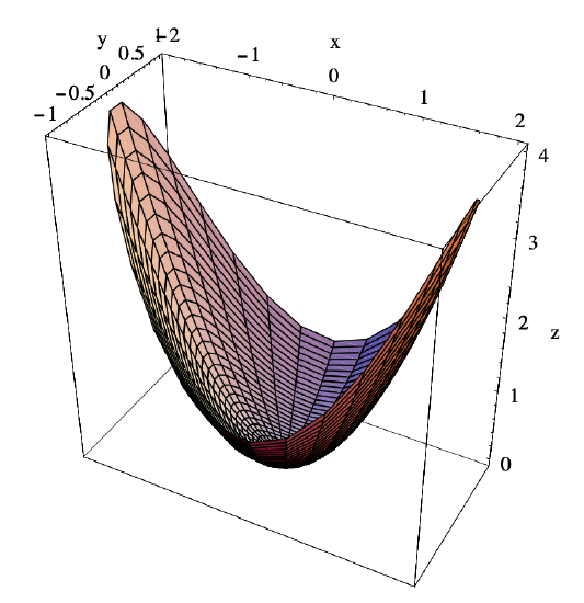
Suppose we wish to find the global extreme values for the function \(f(x,y)=x^2+y^2\) on the closed set

\[ D=\left\{(x, y): x^{2}+4 y^{2} \leq 4\right\} . \nonumber \]

We first find all the critical and singular points. Now

\[ \nabla f(x, y)=(2 x, 2 y) , \nonumber \]

so

\[ \nabla f(x, y)=(0,0) \nonumber \]

if and only if

\[ \begin{aligned}
&2 x=0, \\
&2 y=0.
\end{aligned} \]

Hence the only critical point is (0,0). There are no singular points, but we must consider the boundary of \(S\), the ellipse

\[ B=\left\{(x, y): x^{2}+4 y^{2}=4\right\} . \nonumber \]

Now we may use

\[ \varphi(t)=(2 \cos (t), \sin (t)) , \nonumber \]

\(0 \leq t \leq 2 \pi\), to parametrize \(B\). It follows that any extreme value of \(f\) occurring on \(B\) will also be an extreme value of

\[ \begin{aligned}
g(t) &=f(\varphi(t)) \\
&=f(2 \cos (t), \sin (t)) \\
&=4 \cos ^{2}(t)+\sin ^{2}(t) \\
&=4 \cos ^{2}(t)+\left(1-\cos ^{2}(t)\right) \\
&=3 \cos ^{2}(t)+1
\end{aligned} \]

on the closed interval \([0,2 \pi]\). Now

\[ g^{\prime}(t)=-6 \cos (t) \sin (t) , \nonumber \]

so the critical points of \(g\) occur at points \(t\) in \((0,2 \pi )\) where either \(\cos (t)=0\) or \(\sin (t)=0\). Hence the critical points of \(g\) are \(t=\frac{\pi}{2}\), \(t=\pi\), and \(t=\frac{3 \pi}{2}\). Moreover, we need to consider the endpoints \(t=0\) and \(t=2 \pi \). Hence we have four more candidates for the location of extreme values, namely, \(\varphi(0)=\varphi(2 \pi)=(2,0)\), \(\varphi\left(\frac{\pi}{2}\right)=(0,1)\), \(\varphi(\pi)=(-2,0)\), and \(\varphi\left(\frac{3 \pi}{2}\right)=(0,-1)\). Evaluating \(f\) at these five points, we have

\[ \begin{aligned}
&f(0,0)=0, \\
&f(2,0)=4, \\
&f(0,1)=1, \\
&f(-2,0)=4,
\end{aligned} \]

and

\[ f(0,-1)=1 . \nonumber \]

Comparing these values, we see that \(f\) has a maximum value of 4 at (2,0) and (−2,0) and a minimum value of 0 at (0,0). See Figure 3.5.1 for the graph of \(f\) on the set \(D\).

Figure \(\PageIndex{1}\): Graph of \(f(x, y)=x^{2}+y^{2}\) on \(D=\left\{(x, y): x^{2}+4 y^{2} \leq 4\right\}\)

As the previous example shows, dealing with the boundary of a region can require a significant amount of work. In this example we were helped by the fact that the boundary was one-dimensional and was easily parametrized. This is not always the case. For example, the boundary of the closed ball \(\bar{B}^{3}((0,0,0), 1)\) in \(\mathbb{R}^3\) is the sphere \(S^{2}((0,0,0), 1)\) with equation

\[ x^{2}+y^{2}+z^{2}=1, \nonumber \]

a two-dimensional surface. We shall see in Chapter 4 that it is possible to parametrize such surfaces, but that would still leave us with a two-dimensional problem. We will return to this problem later in this section when we present a much more elegant solution based on our knowledge of level sets and gradient vectors.

Finding local extrema

For now we will turn our attention to identifying local extreme values. Recall from one variable calculus that one of the most useful ways to identify a local extreme value is through the second derivative test. That is, if \(c\) is a critical point of \(\varphi: \mathbb{R} \rightarrow \mathbb{R}\), then \(\varphi^{\prime \prime}(c)>0\) implies that \(\varphi\) has a local minimum at \(c\) and \(\varphi^{\prime \prime}(c)<0\) implies \(\varphi\) has a local maximum at \(c\). Taylor’s theorem provides an easy way to see why this is so. For example, suppose \(c\) is a critical point of \(\varphi\), \(\varphi^{\prime \prime}\) is continuous on an open interval containing \(c\), and \(\varphi^{\prime \prime}(c)>0\). Then there is an interval \(I=(c-r, c+r), r>0\), such that \(\varphi^{\prime \prime}\) is continuous on \(I\) and \(\varphi^{\prime \prime}(t)>0\) for all \(t\) in \(I\). By Taylor’s theorem, for any \(h\) with \(|h|<r\), there is a number \(s\) between \(c\) and \(c+h\) such that

\[ \varphi(c+h)=\varphi(c)+\varphi^{\prime}(c) h+\frac{1}{2} \varphi^{\prime \prime}(s) h^{2}=\varphi(c)+\frac{1}{2} \varphi^{\prime \prime}(s) h^{2}>\varphi(c) , \]

where we have used the fact that \(\varphi^{\prime}(c)=0\) since \(c\) is a critical point of \(\varphi\). Hence \(\varphi (c)\) is a local minimum value of \(\varphi\).

Similar considerations lead to a second derivative test for a function \(f: \mathbb{R}^{n} \rightarrow \mathbb{R}\). Suppose \(\mathbf{c}\) is a critical point of \(f\), \(f\) is \(C^2\) on an open set containing \(\mathbf{c}\), and \(H f(\mathbf{c})\) is positive definite. Let \(B^{n}(\mathbf{c}, r), r>0\), be an open ball on which \(f\) is \(C^2\) and \(H f(\mathbf{c})\) is positive definite. Then, by the version of Taylor’s theorem in Section 3.4, for any \(\mathbf{h}\) with \(\|\mathbf{h}\|<r\), there is a number \(s\) between 0 and 1 such that

\[ f(\mathbf{c}+\mathbf{h})=f(\mathbf{c})+\nabla f(\mathbf{c}) \cdot \mathbf{h}+\frac{1}{2} \mathbf{h}^{T} H f(\mathbf{c}+s \mathbf{h}) \mathbf{h}=f(\mathbf{c})+\frac{1}{2} \mathbf{h}^{T} H f(\mathbf{c}+s \mathbf{h}) \mathbf{h}>f(\mathbf{c}) , \]

where \(\nabla f(\mathbf{c})=\mathbf{0}\) since \(\mathbf{c}\) is a critical point of \(f\), and the final inequality follows from the assumption that \(H f(\mathbf{x})\) is positive definite for \(x\) in \(B^{n}(\mathbf{c}, r)\). Hence \(f(\mathbf{c})\) is a local minimum value of \(f\). The same argument shows that if \(H f(\mathbf{c})\) is negative definite, then \(f(\mathbf{c})\) is a local maximum value of \(f\). If \(H f(\mathbf{c})\) is indefinite, then there will be arbitrarily small \(\mathbf{h}\) for which

\[ \frac{1}{2} \mathbf{h}^{T} H f(\mathbf{c}+s \mathbf{h}) \mathbf{h}>0 \nonumber \]

and arbitrarily small \(\mathbf{h}\) for which

\[ \frac{1}{2} \mathbf{h}^{T} H f(\mathbf{c}+s \mathbf{h}) \mathbf{h}<0 . \nonumber \]

Hence there will be arbitrarily small \(\mathbf{h}\) for which \(f(\mathbf{c}+\mathbf{h})>f(\mathbf{c})\) and arbitrarily small \(\mathbf{h}\) for which \(f(\mathbf{c}+\mathbf{h})<f(\mathbf{c})\). In this case, \(f(\mathbf{c})\) is neither a local minimum nor a local maximum. In this case, we call \(\mathbf{c}\) a saddle point. Finally, if \(H f(\mathbf{c})\) is nondefinite, then we do not have enough information to classify the critical point. We may now state the second derivative test.

Second derivative test

Suppose \(f: \mathbb{R}^{n} \rightarrow \mathbb{R}\) is \(C^2\) on an open set \(U\). If \(\mathbf{c}\) is a critical point of \(f\) in \(U\), then \(f(\mathbf{c})\) is a local minimum value of \(f\) if \(H f(\mathbf{c})\) is positive definite, \(f(\mathbf{c})\) is a local maximum value of \(f\) if \(H f(\mathbf{c})\) is negative definite, and \(\mathbf{c}\) is a saddle point if \(H f(\mathbf{c})\) is indefinite. If \(H f(\mathbf{c})\) is nondefinite, then more information is needed in order to classify \(\mathbf{c}\).

The next example gives an indication for the source of the term saddle point.

Example \(\PageIndex{7}\)

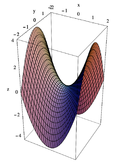
To find the local extreme values of \(f(x, y)=x^{2}-y^{2}\), we begin by finding

\[ \nabla f(x, y)=(2 x,-2 y) . \nonumber \]

Now

\[ \nabla f(x, y)=(0,0) \nonumber \]

if and only if

\[ \begin{aligned}
2 x &=0, \\
-2 y &=0,
\end{aligned} \]

which occurs if and only if \(x=0\) and \(y=0\). Thus \(f\) has the single critical point (0,0). Now

\[ H f(x, y)=\left[\begin{array}{rr}
2 & 0 \\
0 & -2
\end{array}\right], \nonumber \]

so

\[ H f(0,0)=\left[\begin{array}{rr}
2 & 0 \\
0 & -2
\end{array}\right] . \nonumber \]

Thus

\[ \operatorname{det}(H f(0,0))=(2)(-2)=-4<0 . \nonumber \]

Hence \(Hf(0,0)\) is indefinite and so, by the second derivative test, (0,0) is a saddle point. Looking at the graph of \(f\) in Figure 3.5.2, we can see the reason for this: since \(f(x, 0)=x^{2}\) and \(f(0, y)=-y^{2}\), the slice of the graph of \(f\) above the \(x\)-axis is a parabola opening upward while the slice of the graph of \(f\) above the \(y\)-axis is a parabola opening downward.

Figure \(\PageIndex{2}\): Graph of \(f(x, y)=x^{2}-y^{2}\)

Example \(\PageIndex{8}\)

Consider \(f(x, y)=x y e^{-\left(x^{2}+y^{2}\right)}\). Then

\[ \nabla f(x, y)=e^{-\left(x^{2}+y^{2}\right)}\left(y-2 x^{2} y, x-2 x y^{2}\right) . \nonumber \]

Hence, since \(e^{-\left(x^{2}+y^{2}\right)}>0\) for all \((x,y)\),

\[ \nabla f(x, y)=(0,0) \nonumber \]

if and only if

\[ \begin{aligned}
&y-2 x^{2} y=0, \\
&x-2 x y^{2}=0,
\end{aligned} \]

which occurs if and only if

\[ \begin{aligned}
&y\left(1-2 x^{2}\right)=0, \\
&x\left(1-2 y^{2}\right)=0.
\end{aligned} \]

Now the first equation is satisfied if either \(y=0\) or \(1-2 x^{2}=0\). If \(y=0\), then the second equation becomes \(x=0\), so (0,0) is a critical point. If \(1-2 x^{2}=0\), then either \(x=-\frac{1}{\sqrt{2}}\) or \(x=\frac{1}{\sqrt{2}}\). For either of these values of \(x\), the second equation is satisfied if and only if \(1-2 y^{2}=0\), that is, \(y=-\frac{1}{\sqrt{2}}\) or \(y=\frac{1}{\sqrt{2}}\). Hence we have four more critical points: \(\left(-\frac{1}{\sqrt{2}},-\frac{1}{\sqrt{2}}\right),\left(-\frac{1}{\sqrt{2}}, \frac{1}{\sqrt{2}}\right),\left(\frac{1}{\sqrt{2}},-\frac{1}{\sqrt{2}}\right)\), and \(\left(\frac{1}{\sqrt{2}}, \frac{1}{\sqrt{2}}\right)\). Now

\[ H f(x, y)=e^{-\left(x^{2}+y^{2}\right)}\left[\begin{array}{cc}
4 x^{3} y-6 x y & 4 x^{2} y^{2}-2 x^{2}-2 y^{2}+1 \\
4 x^{2} y^{2}-2 x^{2}-2 y^{2}+1 & 4 y^{3} x-6 x y
\end{array}\right] , \nonumber \]

so

\[ \begin{gathered}
H f(0,0)=\left[\begin{array}{ll}
0 & 1 \\
1 & 0
\end{array}\right], \\
H f\left(-\frac{1}{\sqrt{2}},-\frac{1}{\sqrt{2}}\right)=H f\left(\frac{1}{\sqrt{2}}, \frac{1}{\sqrt{2}}\right)=e^{-1}\left[\begin{array}{rr}
-2 & 0 \\
0 & -2
\end{array}\right],
\end{gathered}\]

and

\[ H f\left(-\frac{1}{\sqrt{2}}, \frac{1}{\sqrt{2}}\right)=H f\left(\frac{1}{\sqrt{2}},-\frac{1}{\sqrt{2}}\right)=e^{-1}\left[\begin{array}{ll}
2 & 0 \\
0 & 2
\end{array}\right] . \nonumber \]

Since

\[ \begin{gathered}
\operatorname{det}\left[\begin{array}{ll}
0 & 1 \\
1 & 0
\end{array}\right]=-1<0, \\
\operatorname{det}\left[\begin{array}{cc}
-2 e^{-1} & 0 \\
0 & -2 e^{-1}
\end{array}\right]=4 e^{-2}>0,
\end{gathered}\]

and

\[ \operatorname{det}\left[\begin{array}{cc}
2 e^{-1} & 0 \\
0 & 2 e^{-1}
\end{array}\right]=4 e^{-2}>0 , \nonumber \]

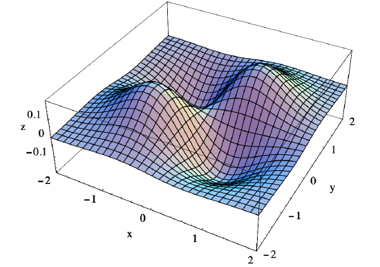
we see that \(Hf(0,0)\) is indefinite, \(H f\left(-\frac{1}{\sqrt{2}},-\frac{1}{\sqrt{2}}\right)\) and \(H f\left(\frac{1}{\sqrt{2}}, \frac{1}{\sqrt{2}}\right)\) are negative definite, and \(H f\left(-\frac{1}{\sqrt{2}}, \frac{1}{\sqrt{2}}\right)\) and \(H f\left(-\frac{1}{\sqrt{2}}, \frac{1}{\sqrt{2}}\right)\) are positive definite. Thus (0,0) is a saddle point of \(f\), \(f\) has local maximums of \(\frac{1}{2} e^{-1}\) at both \(\left(-\frac{1}{\sqrt{2}},-\frac{1}{\sqrt{2}}\right)\) and \(\left(\frac{1}{\sqrt{2}}, \frac{1}{\sqrt{2}}\right)\), and local minimums of \(-\frac{1}{2} e^{-1}\) at \(\left(-\frac{1}{\sqrt{2}}, \frac{1}{\sqrt{2}}\right)\) and \(\left(\frac{1}{\sqrt{2}},-\frac{1}{\sqrt{2}}\right)\). See Figure 3.5.3.

Figure \(\PageIndex{3}\): Graph of \(f(x, y)=x y e^{-\left(x^{2}+y^{2}\right)}\)

Finding global extrema

The graph of \(f(x, y)=x y e^{-\left(x^{2}+y^{2}\right)}\) in Figure 3.5.3 suggests that local extreme values found in the previous example are in fact global extreme values for \(f\) on all of \(\mathbb{R}^2\). We may verify that this in fact the case as follows. First note that, since

\[ \lim _{r \rightarrow \infty} r^{2} e^{-r^{2}}=0 , \nonumber \]

we may choose \(R\) large enough so that

\[ r^{2} e^{-r^{2}}<\frac{1}{2} e^{-1} \nonumber \]

whenever \(r \geq R\). Now for any point \((x,y)\) with \(\|(x, y)\|=r \geq R\) we have

\[ |f(x, y)|=\left|x y e^{-\left(x^{2}+y^{2}\right)}\right|=|x||y| e^{-\left(x^{2}+y^{2}\right)} \leq r^{2} e^{-r^{2}}<\frac{1}{2} e^{-1} . \nonumber \]

Hence \(f(x,y)\) is between \(-\frac{1}{2} e^{-1}\) and \(\frac{1}{2} e^{-1}\) for all points \((x,y)\) outside of the closed disk \(D=\bar{B}^{2}((0,0), R)\). Moreover, since \(f(x,y)\) is between \(-\frac{1}{2} e^{-1}\) and \(\frac{1}{2} e^{-1}\) for all points \((x,y)\) on the boundary of \(D\), \(f\) has a minimum value of \(-\frac{1}{2} e^{-1}\) and a maximum value of \(\frac{1}{2} e^{-1}\) on \(D\). Hence these values are actually the global extreme values of \(f\) on all of \(\mathbb{R}^2\).

Example \(\PageIndex{9}\)

A farmer wishes to build a rectangular storage bin, without a top, with a volume of 500 cubic meters using the least amount of material possible. If we let \(x\) and \(y\) be the dimensions of the base of the bin and \(z\) be the height, all measured in meters, then the farmer wishes to minimize the surface area of the bin, given by

\[ S=x y+2 x z+2 y z , \label{3.5.3} \]

subject to the constraint on the volume, namely,

\[ 500=x y z . \nonumber \]

Solving for \(z\) in the latter expression and substituting in to (\(\ref{3.5.3}\)), we have

\[ S=x y+2 x\left(\frac{500}{x y}\right)+2 y\left(\frac{500}{x y}\right)=x y+\frac{1000}{y}+\frac{1000}{x} . \nonumber \]

This is the function we need to minimize on the infinite open rectangle

\[ R=\{(x, y): x>0, y>0\} . \nonumber \]

Now

\[ \frac{\partial S}{\partial x}=y-\frac{1000}{x^{2}} \nonumber \]

and

\[ \frac{\partial S}{\partial y}=x-\frac{1000}{y^{2}} \nonumber \]

so to find the critical points of \(S\) we need to solve

\[ \begin{aligned}
&y-\frac{1000}{x^{2}}=0, \\
&x-\frac{1000}{y^{2}}=0.
\end{aligned}\]

Solving for \(y\) in the first of these, we have

\[ y=\frac{1000}{x^{2}} , \nonumber \]

which, when substituted into the second, gives us

\[ x-\frac{x^{4}}{1000}=0 . \nonumber \]

Hence we want

\[ x\left(1-\frac{x^{3}}{1000}\right)=0 , \nonumber \]

from which it follows that either \(x = 0\) or \(x = 10\). Since the first of these will not give us a point in \(R\), we have \(x = 10\) and

\[ y=\frac{1000}{10^{2}}=10 . \nonumber \]

Thus the only critical point is (10,10). Now

\[ H S(x, y)=\left[\begin{array}{cc}
\frac{2000}{x^{3}} & 1 \\
1 & \frac{2000}{y^{3}}
\end{array}\right] , \nonumber \]

so

\[ H S(10,10)=\left[\begin{array}{ll}
2 & 1 \\
1 & 2
\end{array}\right] . \nonumber \]

Thus

\[ \operatorname{det}(H S(10,10))=3 , \nonumber \]

and so \(HS(10,10)\) is positive definite. This shows that \(S\) has a local minimum of

\[ \left.S\right|_{x=10, y=10}=(10)(10)+\frac{1000}{10}+\frac{1000}{10}=300 \nonumber \]

at \((x, y)=(10,10)\). To show that this is actually the global minimum value of \(S\), we proceed as follows. Let \(D\) be the closed rectangle

\[ D=\{(x, y): 1 \leq x \leq 400,1 \leq y \leq 400\} . \nonumber \]

Now if \(0<x \leq 1\), then

\[ \frac{1000}{x} \geq 1000 , \nonumber \]

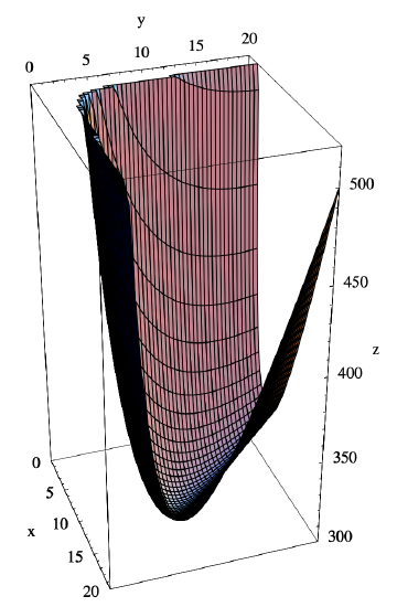
and so \(S > 300\). Similarly, if \(0<y \leq 1\), then \(S > 300\). Moreover, if \(x \geq 400\) and \(y \geq 1\), then \(xy \geq 400\), and so \(S > 300\). Similarly, if \(y \geq 400\) and \(x \geq 1\), then \(S > 300\). Hence \(S > 300\) for all \((x,y)\) outside of \(D\) and for all \((x,y)\) on the boundary of \(D\). Hence \(S\) has a global minimum of 300 on \(D\), which, from the preceding observations, must in fact be the global minimum of \(S\) on all of \(R\). See the graph of \(S\) in Figure 3.5.4. Finally, when \(x=10\) and \(y=10\), we have

\[ z=\frac{500}{(10)(10)}=5 , \nonumber \]

so the farmer should build her bin to have a base of 10 meters by 10 meters and a height of 5 meters.

Figure \(\PageIndex{4}\): Graph of \(S=x y+\frac{1000}{x}+\frac{1000}{y}\)

Lagrange multipliers

This last example has much in common with our first example in that they both involve finding extreme values of a function restricted to a lower-dimensional subset. In our first example, we had to find the extreme values of \(f(x, y)=x^{2}+y^{2}\) restricted to the one dimensional ellipse with equation \(x^{2}+4 y^{2}=4\); in the example we just finished, we had to find the minimum value of \(S=x y+2 x z+2 y z\), a function of three variables, restricted to the two-dimensional surface defined by the equation \(xyz = 500\). Although they were similar, we approached these problems somewhat differently. In the first, we parametrized the ellipse and then maximized the composition of \(f\) with this parametrization; in the latter, we solved for \(z\) in terms of \(x\) and \(y\) and then substituted into the formula for \(S\) to make \(S\) effectively a function of two variables. Now we will describe a general approach which applies to both situations. Often, but not always, this method is easier to apply then the other two techniques. In practice, one tries to select the method that will yield an answer with the least resistance.

For the general case, consider two differentiable functions, \(f: \mathbb{R}^{n} \rightarrow \mathbb{R}\) and \(g: \mathbb{R}^{n} \rightarrow \mathbb{R}\), and suppose we wish to find the extreme values of \(f\) on the level set \(S\) of \(g\) determined by the constraint \(g(\mathbf{x})=0\). If \(f\) has an extreme value at a point \(\mathbf{c}\) on \(S\), then \(f(\mathbf{c})\) must be an extreme value of \(f\) along any curve passing through \(\mathbf{c}\). Thus if \(\varphi: \mathbb{R} \rightarrow \mathbb{R}^{n}\) parametrizes a curve in \(S\) with \(\varphi(b)=\mathbf{c}\), then the function \(h(t)=f(\varphi(t))\) has an extreme value at \(b\). Hence

\[ 0=h^{\prime}(b)=\nabla f(\varphi(b)) \cdot D \varphi(b)=\nabla f(\mathbf{c}) \cdot D \varphi(b) . \label{3.5.4} \]

Since (\(\ref{3.5.4}\)) holds for any curve in \(S\) through \(\mathbf{c}\) and \(D \varphi(b)\) is tangent to the given curve at \(\mathbf{c}\), it follows that \(\nabla f(\mathbf{c})\) is orthogonal to the tangent hyperplane to \(S\) at \(\mathbf{c}\). But \(S\) is a level set of \(g\), so we know from our work in Section 3.3 that the vector \(\nabla g(\mathbf{c})\), provided it is nonzero, is a normal vector for the tangent hyperplane to \(S\) at \(\mathbf{c}\). Hence \nabla f(\mathbf{c}) and \nabla g(\mathbf{c}) must be parallel. That is, there must exist a scalar \(\lambda\) such that

\[ \nabla f(\mathbf{c})=\lambda \nabla g(\mathbf{c}) . \]

The idea now is that in looking for extreme values, we need only consider points \(\mathbf{c}\) for which both \(g(\mathbf{c})=0\) and \(\nabla f( \mathbf{c} )= \lambda \nabla g( \mathbf{c} ) \) for some scalar \( \lambda \). The scalar \( \lambda \) is known as a Lagrange multiplier, and this method for finding extreme values subject to a constraining equation is known as the method of Lagrange multipliers.

Example \(\PageIndex{10}\)

Suppose that the temperature at a point \((x,y,z)\) on the unit sphere \(S =S^{2}((0,0,0), 1)\) is given by

\[ T(x, y, z)=30+5(x+z) . \nonumber \]

To find the extreme values of \(T\), we first define

\[ g(x, y, z)=x^{2}+y^{2}+z^{2}-1, \nonumber \]

thus making \(S\) the level surface of \(g\) specified by \(g(x,y,z) = 0\). Now

\[ \nabla f(x, y, z)=(5,0,5) \nonumber \]

and

\[ \nabla g(x, y, z)=(2 x, 2 y, 2 z) . \nonumber \]

The candidates for the locations of extreme values will be solutions of the equations

\[ \begin{aligned}
\nabla f(x, y, z) &=\lambda \nabla g(x, y, z), \\
g(x, y, z) &=0,
\end{aligned} \]

that is,

\[ \begin{aligned}
&(5,0,5)=\lambda(2 x, 2 y, 2 z), \\
&x^{2}+y^{2}+z^{2}-1=0 .
\end{aligned} \]

Hence we need to solve the following system of four equation in four unknowns:

\[ \begin{gathered}
5=2 \lambda x, \\
0=2 \lambda y, \\
5=2 \lambda z, \\
x^{2}+y^{2}+z^{2}=1.
\end{gathered} \]

Now \(5 = 2 \lambda x\) implies that \(\lambda \neq 0,\) and so \(0=2 \lambda y\) implies that \(y=0\). Moreover, \(5 = 2 \lambda x\) and \(5 = 2 \lambda z\) imply that \(2 \lambda x = 2 \lambda z \), from which it follows, since \(\lambda \neq 0,\), that \(x=z\). Substituting these results into the final equation, we have

\[ 1=x^{2}+y^{2}+z^{2}=x^{2}+0+x^{2}=2 x^{2} . \nonumber \]

Thus \( x=-\frac{1}{\sqrt{2}} \) or \(x=\frac{1}{\sqrt{2}}\), and we have two solutions for our equations,

\[ \left(-\frac{1}{\sqrt{2}}, 0,-\frac{1}{\sqrt{2}}\right) \nonumber \]

and

\[ \left(\frac{1}{\sqrt{2}}, 0, \frac{1}{\sqrt{2}}\right) \nonumber \]

At this point, since \(T\) is continuous and \(S\) is closed and bounded, we need only evaluate \(T\) at these points and compare their values. Now

\[ T\left(-\frac{1}{\sqrt{2}}, 0,-\frac{1}{\sqrt{2}}\right)=30-5 \sqrt{2}=22.93 \nonumber \]

and

\[ T\left(\frac{1}{\sqrt{2}}, 0, \frac{1}{\sqrt{2}}\right)=30+5 \sqrt{2}=37.07 , \nonumber \]

where the final values have been rounded to two decimal places, so the maximum temperature on the sphere is 37.07 at \(\left(\frac{1}{\sqrt{2}}, 0, \frac{1}{\sqrt{2}}\right)\) and the minimum temperature is 22.93 at \(\left(-\frac{1}{\sqrt{2}}, 0,-\frac{1}{\sqrt{2}}\right)\).

Example \(\PageIndex{11}\)

Suppose the farmer in our earlier example is faced with the opposite problem: Given 300 square meters of material, what are the dimensions of the rectangular bin, without a top, that holds the largest volume? If we again let \(x\) and \(y\) be the dimensions of the base of the bin and \(z\) be its height, then we want to maximize

\[ V=x y z \nonumber \]

on the region where \(x>0, y>0\), and \(z>0\), subject to the constraint that

\[ x y+2 x z+2 y z=300 . \nonumber \]

If we let

\[ g(x, y, z)=x y+2 x z+2 y z-300 , \nonumber \]

then our problem is to maximize \(V\) subject to the constraint \(g(x, y, z)=0\). Now

\[ \nabla V=(y z, x z, x y) \nonumber \]

and

\[ \nabla g(x, y, z)=(y+2 z, x+2 z, 2 x+2 y) , \nonumber \]

so the system of equations

\[ \begin{gathered}
\nabla V=\lambda \nabla g(x, y, z), \\
g(x, y, z)=0,
\end{gathered} \]

becomes the system

\[ \begin{align}
y z=\lambda(y+2 z), \label{3.5.6} \\
x z=\lambda(x+2 z), \label{3.5.7} \\
x y=\lambda(2 x+2 y), \label{3.5.8} \\
x y+2 x z+2 y z=300 . \label{3.5.9}
\end{align} \]

Equations (\(\ref{3.5.6}\)) and (\(\ref{3.5.7}\)) imply that

\[ \lambda=\frac{y x}{y+2 z} \nonumber \]

and

\[ \lambda=\frac{x z}{x+2 z} , \nonumber \]

so

\[ \frac{y z}{y+2 z}=\frac{x z}{x+2 z} , \nonumber \]

that is,

\[ \frac{y}{y+2 z}=\frac{x}{x+2 z} . \nonumber \]

Hence

\[ x y+2 y z=x y+2 x z . \nonumber \]

Thus \(2 y z=2 x z\), so \(x=y\). Substituting this result into (\(\ref{3.5.8}\)) gives us \(x^{2}=4 \lambda x\), from which it follows that \( x = 4 \lambda \). Substituting into (\(\ref{3.5.7}\)), we have

\[ 4 \lambda z=\lambda(4 \lambda+2 z)=4 \lambda^{2}+2 \lambda z . \nonumber \]

Hence \(2 \lambda z=4 \lambda^{2}\), so \(z = 2 \lambda \). Putting \( x = 4 \lambda \), \( y = 4 \lambda \), and \(z = 2 \lambda \) into (\(\ref{3.5.9}\)) yields the equation

\[ 16 \lambda^{2}+16 \lambda^{2}+16 \lambda^{2}=300 . \nonumber \]

Thus \(48 \lambda^{2}=300\), so

\[ \lambda=\pm \sqrt{\frac{300}{48}}=\pm \sqrt{\frac{25}{4}}=\pm \frac{5}{2} . \nonumber \]

Now \(x\), \(y\), and \(z\) are all positive, so we must have \(\lambda=\frac{5}{2}\), giving us \(x=10\), \(y=10\), and \(z=5\). To show that we have the location of the maximum value of \(V\), let

\[ S=\{(x, y, z): g(x, y, z)=0, x>0, y>0, z>0\} \nonumber \]

and let \(D\) be that part of \(S\) for which \( 1 \leq x \leq 150\), \( 1 \leq y \leq 150\), and \( 1 \leq z \leq 150\). Note that if \((x,y,z)\) lies on \(S\), then

\[ 300=x y+2 x z+2 y z \nonumber \]

and so \( xy \leq 300\), \( xz \leq 150\), and \( yz \leq 150\). Moreover,

\[ z=\frac{300-x y}{2 x+2 y} . \nonumber \]

Now if either \( x \geq 150\) or \( y \geq 150\), then

\[ z \leq \frac{300}{300} \leq 1 , \nonumber \]

so

\[ V=x y z \leq(300)(1)=300 . \nonumber \]

If \(x \leq 1\),

\[ V=x y z \leq(1)(150)=150 \nonumber \]

and, similarly, if \(y \leq 1 \),

\[ V=y x z \leq(1)(150)=150 . \nonumber \]

Thus if \((x,y,z)\) is either on the boundary of \(D\) or outside of \(D\), then \(V \leq 300\). Since

\[ \left.V\right|_{(x, y, z)=(10,10,5)}=500 , \nonumber \]

it follows that the global maximum of \(V\) on \(S\) must occur inside \(D\). In fact, this maximum value must be 500 cubic meters, occurring when \(x=10\) meters, \(y=10\) meters, and \(z=5\) meters.