Mathematics LibreTexts

3.4: Numerical Approximation of Multiple Integrals

  • Page ID
    2245
  • \( \newcommand{\vecs}[1]{\overset { \scriptstyle \rightharpoonup} {\mathbf{#1}} } \)

    \( \newcommand{\vecd}[1]{\overset{-\!-\!\rightharpoonup}{\vphantom{a}\smash {#1}}} \)

    \( \newcommand{\id}{\mathrm{id}}\) \( \newcommand{\Span}{\mathrm{span}}\)

    ( \newcommand{\kernel}{\mathrm{null}\,}\) \( \newcommand{\range}{\mathrm{range}\,}\)

    \( \newcommand{\RealPart}{\mathrm{Re}}\) \( \newcommand{\ImaginaryPart}{\mathrm{Im}}\)

    \( \newcommand{\Argument}{\mathrm{Arg}}\) \( \newcommand{\norm}[1]{\| #1 \|}\)

    \( \newcommand{\inner}[2]{\langle #1, #2 \rangle}\)

    \( \newcommand{\Span}{\mathrm{span}}\)

    \( \newcommand{\id}{\mathrm{id}}\)

    \( \newcommand{\Span}{\mathrm{span}}\)

    \( \newcommand{\kernel}{\mathrm{null}\,}\)

    \( \newcommand{\range}{\mathrm{range}\,}\)

    \( \newcommand{\RealPart}{\mathrm{Re}}\)

    \( \newcommand{\ImaginaryPart}{\mathrm{Im}}\)

    \( \newcommand{\Argument}{\mathrm{Arg}}\)

    \( \newcommand{\norm}[1]{\| #1 \|}\)

    \( \newcommand{\inner}[2]{\langle #1, #2 \rangle}\)

    \( \newcommand{\Span}{\mathrm{span}}\) \( \newcommand{\AA}{\unicode[.8,0]{x212B}}\)

    \( \newcommand{\vectorA}[1]{\vec{#1}}      % arrow\)

    \( \newcommand{\vectorAt}[1]{\vec{\text{#1}}}      % arrow\)

    \( \newcommand{\vectorB}[1]{\overset { \scriptstyle \rightharpoonup} {\mathbf{#1}} } \)

    \( \newcommand{\vectorC}[1]{\textbf{#1}} \)

    \( \newcommand{\vectorD}[1]{\overrightarrow{#1}} \)

    \( \newcommand{\vectorDt}[1]{\overrightarrow{\text{#1}}} \)

    \( \newcommand{\vectE}[1]{\overset{-\!-\!\rightharpoonup}{\vphantom{a}\smash{\mathbf {#1}}}} \)

    \( \newcommand{\vecs}[1]{\overset { \scriptstyle \rightharpoonup} {\mathbf{#1}} } \)

    \( \newcommand{\vecd}[1]{\overset{-\!-\!\rightharpoonup}{\vphantom{a}\smash {#1}}} \)

    \(\newcommand{\avec}{\mathbf a}\) \(\newcommand{\bvec}{\mathbf b}\) \(\newcommand{\cvec}{\mathbf c}\) \(\newcommand{\dvec}{\mathbf d}\) \(\newcommand{\dtil}{\widetilde{\mathbf d}}\) \(\newcommand{\evec}{\mathbf e}\) \(\newcommand{\fvec}{\mathbf f}\) \(\newcommand{\nvec}{\mathbf n}\) \(\newcommand{\pvec}{\mathbf p}\) \(\newcommand{\qvec}{\mathbf q}\) \(\newcommand{\svec}{\mathbf s}\) \(\newcommand{\tvec}{\mathbf t}\) \(\newcommand{\uvec}{\mathbf u}\) \(\newcommand{\vvec}{\mathbf v}\) \(\newcommand{\wvec}{\mathbf w}\) \(\newcommand{\xvec}{\mathbf x}\) \(\newcommand{\yvec}{\mathbf y}\) \(\newcommand{\zvec}{\mathbf z}\) \(\newcommand{\rvec}{\mathbf r}\) \(\newcommand{\mvec}{\mathbf m}\) \(\newcommand{\zerovec}{\mathbf 0}\) \(\newcommand{\onevec}{\mathbf 1}\) \(\newcommand{\real}{\mathbb R}\) \(\newcommand{\twovec}[2]{\left[\begin{array}{r}#1 \\ #2 \end{array}\right]}\) \(\newcommand{\ctwovec}[2]{\left[\begin{array}{c}#1 \\ #2 \end{array}\right]}\) \(\newcommand{\threevec}[3]{\left[\begin{array}{r}#1 \\ #2 \\ #3 \end{array}\right]}\) \(\newcommand{\cthreevec}[3]{\left[\begin{array}{c}#1 \\ #2 \\ #3 \end{array}\right]}\) \(\newcommand{\fourvec}[4]{\left[\begin{array}{r}#1 \\ #2 \\ #3 \\ #4 \end{array}\right]}\) \(\newcommand{\cfourvec}[4]{\left[\begin{array}{c}#1 \\ #2 \\ #3 \\ #4 \end{array}\right]}\) \(\newcommand{\fivevec}[5]{\left[\begin{array}{r}#1 \\ #2 \\ #3 \\ #4 \\ #5 \\ \end{array}\right]}\) \(\newcommand{\cfivevec}[5]{\left[\begin{array}{c}#1 \\ #2 \\ #3 \\ #4 \\ #5 \\ \end{array}\right]}\) \(\newcommand{\mattwo}[4]{\left[\begin{array}{rr}#1 \amp #2 \\ #3 \amp #4 \\ \end{array}\right]}\) \(\newcommand{\laspan}[1]{\text{Span}\{#1\}}\) \(\newcommand{\bcal}{\cal B}\) \(\newcommand{\ccal}{\cal C}\) \(\newcommand{\scal}{\cal S}\) \(\newcommand{\wcal}{\cal W}\) \(\newcommand{\ecal}{\cal E}\) \(\newcommand{\coords}[2]{\left\{#1\right\}_{#2}}\) \(\newcommand{\gray}[1]{\color{gray}{#1}}\) \(\newcommand{\lgray}[1]{\color{lightgray}{#1}}\) \(\newcommand{\rank}{\operatorname{rank}}\) \(\newcommand{\row}{\text{Row}}\) \(\newcommand{\col}{\text{Col}}\) \(\renewcommand{\row}{\text{Row}}\) \(\newcommand{\nul}{\text{Nul}}\) \(\newcommand{\var}{\text{Var}}\) \(\newcommand{\corr}{\text{corr}}\) \(\newcommand{\len}[1]{\left|#1\right|}\) \(\newcommand{\bbar}{\overline{\bvec}}\) \(\newcommand{\bhat}{\widehat{\bvec}}\) \(\newcommand{\bperp}{\bvec^\perp}\) \(\newcommand{\xhat}{\widehat{\xvec}}\) \(\newcommand{\vhat}{\widehat{\vvec}}\) \(\newcommand{\uhat}{\widehat{\uvec}}\) \(\newcommand{\what}{\widehat{\wvec}}\) \(\newcommand{\Sighat}{\widehat{\Sigma}}\) \(\newcommand{\lt}{<}\) \(\newcommand{\gt}{>}\) \(\newcommand{\amp}{&}\) \(\definecolor{fillinmathshade}{gray}{0.9}\)

    As you have seen, calculating multiple integrals is tricky even for simple functions and regions. For complicated functions, it may not be possible to evaluate one of the iterated integrals in a simple closed form. Luckily there are numerical methods for approximating the value of a multiple integral. The method we will discuss is called the Monte Carlo method. The idea behind it is based on the concept of the average value of a function, which you learned in single-variable calculus. Recall that for a continuous function \(f (x)\), the average value \(\bar f \text{ of }f\) over an interval \([a,b]\) is defined as

    \[\bar f = \dfrac{1}{b-a}\int_a^b f (x)\,dx \label{Eq3.11}\]

    The quantity \(b − a\) is the length of the interval \([a,b]\), which can be thought of as the “volume” of the interval. Applying the same reasoning to functions of two or three variables, we define the average value of \(f (x, y)\) over a region \(R\) to be

    \[\bar f = \dfrac{1}{A(R)} \iint\limits_R f (x, y)\,d A \label{Eq3.12}\]

    where \(A(R)\) is the area of the region \(R\), and we define the average value of \(f (x, y, z)\) over a solid \(S\) to be

    \[\bar f = \dfrac{1}{V(S)} \iiint\limits_S f (x, y, z)\,dV \label{Eq3.13}\]

    where \(V(S)\) is the volume of the solid \(S\). Thus, for example, we have

    \[\iint\limits_R f (x, y)\,d A = A(R) \bar f \label{Eq3.14}\]

    The average value of \(f (x, y)\) over \(R\) can be thought of as representing the sum of all the values of \(f\) divided by the number of points in \(R\). Unfortunately there are an infinite number (in fact, uncountably many) points in any region, i.e. they can not be listed in a discrete sequence. But what if we took a very large number \(N\) of random points in the region \(R\) (which can be generated by a computer) and then took the average of the values of \(f\) for those points, and used that average as the value of \(\bar f\) ? This is exactly what the Monte Carlo method does. So in Formula \ref{Eq3.14} the approximation we get is

    \[\iint\limits_R f (x, y)\,d A \approx A(R) \bar f \pm A(R) \sqrt{\dfrac{\bar {f^2}-(\bar f)^2}{N}}\label{Eq3.15}\]

    where

    \[\bar f = \dfrac{\sum_{i=1}^{N}f(x_i,y_i)}{N}\text{ and } \bar {f^2} = \dfrac{\sum_{i=1}^{N}(f(x_i,y_i))^2}{N}\label{Eq3.16}\]

    with the sums taken over the \(N\) random points \((x_1 , y_1), ..., (x_N , y_N )\). The \(\pm\) “error term” in Formula \ref{Eq3.15} does not really provide hard bounds on the approximation. It represents a single standard deviation from the expected value of the integral. That is, it provides a likely bound on the error. Due to its use of random points, the Monte Carlo method is an example of a probabilistic method (as opposed to deterministic methods such as Newton’s method, which use a specific formula for generating points).

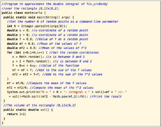
    For example, we can use Formula \ref{Eq3.15} to approximate the volume \(V\) under the plane \(z = 8x + 6y\) over the rectangle \(R = [0,1] \times [0,2]\). In Example 3.1 in Section 3.1, we showed that the actual volume is 20. Below is a code listing (montecarlo.java) for a Java program that calculates the volume, using a number of points \(N\) that is passed on the command line as a parameter.

    alt

    Listing 3.1 Program listing for montecarlo.java

    The results of running this program with various numbers of random points (e.g. java montecarlo 100) are shown below:

    alt

    As you can see, the approximation is fairly good. As \(N \to \infty\), it can be shown that the Monte Carlo approximation converges to the actual volume (on the order of \(O( \sqrt{N})\), in computational complexity terminology).

    In the above example the region \(R\) was a rectangle. To use the Monte Carlo method for a nonrectangular (bounded) region \(R\), only a slight modification is needed. Pick a rectangle \(\tilde R \text{ that encloses }R\), and generate random points in that rectangle as before. Then use those points in the calculation of \(\bar f\) only if they are inside \(R\). There is no need to calculate the area of \(R\) for Equation \ref{Eq3.15} in this case, since the exclusion of points not inside \(R\) allows you to use the area of the rectangle \(\tilde R\) instead, similar to before.

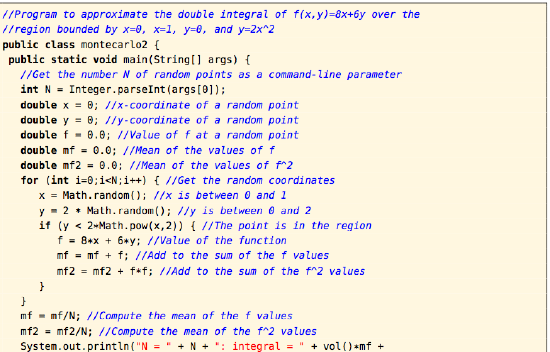
    For instance, in Example 3.4 we showed that the volume under the surface \(z = 8x + 6y\) over the nonrectangular region \(R = {(x, y) : 0 ≤ x ≤ 1, 0 ≤ y ≤ 2x^2 }\) is 6.4. Since the rectangle \(\tilde R = [0,1] \times [0,2] \text{ contains }R\), we can use the same program as before, with the only change being a check to see if \(y < 2x^2\) for a random point \((x, y) \text{ in }[0,1] \times [0,2]\). Listing 3.2 below contains the code (montecarlo2.java):
    alt

    alt

    Listing 3.2 Program listing for montecarlo2.java

    The results of running the program with various numbers of random points (e.g. java montecarlo2 1000) are shown below:

    alt

    To use the Monte Carlo method to evaluate triple integrals, you will need to generate random triples \((x, y, z)\) in a parallelepiped, instead of random pairs \((x, y)\) in a rectangle, and use the volume of the parallelepiped instead of the area of a rectangle in Equation \ref{Eq3.15} (see Exercise 2). For a more detailed discussion of numerical integration methods, see PRESS et al.


    This page titled 3.4: Numerical Approximation of Multiple Integrals is shared under a GNU Free Documentation License 1.3 license and was authored, remixed, and/or curated by Michael Corral via source content that was edited to the style and standards of the LibreTexts platform.

    • Was this article helpful?