3.5: Change of Variables in Multiple Integrals

Given the difficulty of evaluating multiple integrals, the reader may be wondering if it is possible to simplify those integrals using a suitable substitution for the variables. The answer is yes, though it is a bit more complicated than the substitution method which you learned in single-variable calculus.

Recall that if you are given, for example, the definite integral

\[ \int_1^2 x^3 \sqrt{x^2-1}\,dx \]

then you would make the substitution

\[\begin{align} u &= x^2-1 \Rightarrow x^2=u+1 \\[4pt] \nonumber du &= 2x\,dx \end{align}\]

which changes the limits of integration

\[ \begin{align} x &=1 \Rightarrow u=0 \\[4pt] \nonumber x&=2 \Rightarrow u=3 \end{align}\]

so that we get

\[\nonumber \begin{align} \int_1^2 x^3 \sqrt{x^2-1} &= \int_1^2 \dfrac{1}{2}x^2 \cdot 2x\sqrt{x^2-1}\,dx \\[4pt] \nonumber &=\int_0^3 \dfrac{1}{2}(u+1)\sqrt{u}\,du \\[4pt] \nonumber &=\dfrac{1}{2}\int_0^3 \left ( u^{3/2}+u^{1/2} \right )\,du,\text{ which can be easily integrated to give} \\[4pt] \nonumber &=\dfrac{14\sqrt{3}}{5} \end{align} \]

Let us take a different look at what happened when we did that substitution, which will give some motivation for how substitution works in multiple integrals. First, we let \(u = x^2 − 1\). On the interval of integration \([1,2]\), the function \(x \mapsto x^2 −1\) is strictly increasing (and maps \([1,2] \text{ onto }[0,3])\) and hence has an inverse function (defined on the interval \([0,3]\)). That is, on \([0,3]\) we can define \(x\text{ as a function of }u\), namely

\[x=g(u) = \sqrt{u+1}\]

Then substituting that expression for \(x\) into the function \(f (x) = x^3 \sqrt{x^2 −1}\) gives

\[ f (x) = f (g(u)) = (u +1)^{3/2}\sqrt{u}\]

and we see that

\[ \begin{align} \dfrac{dx}{du} = g'(u) \Rightarrow dx &= g'(u)\,du \\[4pt] \nonumber dx &= \dfrac{1}{2}(u+1)^{-1/2}\,du \end{align}\]

so since

\[ \begin{align} g(0) = 1 \Rightarrow 0 &=g^{-1}(1) \\[4pt] \nonumber g(3) =2 \Rightarrow 3 &= g^{-1}(2) \end{align}\]

then performing the substitution as we did earlier gives

\[ \begin{align} \int_1^2 f(x)\,dx &= \int_1^2 x^3 \sqrt{x^2-1}\,dx \\[4pt] \nonumber &=\int_0^3 \dfrac{1}{2}(u+1)\sqrt{u}\,du,\text {which can be written as} \\[4pt] \nonumber &=\int_0^3 (u+1)^{3/2}\sqrt{u}\cdot \dfrac{1}{2}(u+1)^{-1/2}\,du, \text{ which means} \\[4pt] \nonumber \int_1^2 f(x)\,dx &= \int_{g^{-1}(1)}^{g^{-1}(2)} f(g(u))g'(u)\,du \end{align}\]

In general, if \(x = g(u)\) is a one-to-one, differentiable function from an interval \([c,d]\) (which you can think of as being on the “\(u\)-axis”) onto an interval \([a,b]\) (on the \(x\)-axis), which means that \(g′(u) \neq 0\) on the interval \((c,d)\), so that \(a = g(c)\text{ and }b = g(d),\text{ then }c = g^{ −1} (a)\text{ and }d = g^{−1} (b)\), and

\[\int_a^b f(x)\,dx = \int_{g^{-1}(a)}^{g^{-1}(b)} f(g(u))g'(u)\,du \label{Eq3.17}\]

This is called the change of variable formula for integrals of single-variable functions, and it is what you were implicitly using when doing integration by substitution. This formula turns out to be a special case of a more general formula which can be used to evaluate multiple integrals. We will state the formulas for double and triple integrals involving real-valued functions of two and three variables, respectively. We will assume that all the functions involved are continuously differentiable and that the regions and solids involved all have “reasonable” boundaries. The proof of the following theorem is beyond the scope of the text.

Theorem \(\PageIndex{1}\): Change of Variables Formula for Multiple Integrals

Let \(x = x(u,v) \text{ and }y = y(u,v)\) define a one-to-one mapping of a region \(R ′\) in the \(uv\)-plane onto a region \(R\) in the \(x y\)-plane such that the determinant

\[J(u,v) = \begin{vmatrix} \dfrac{∂x}{∂u} & \dfrac{∂x}{∂v} \\[4pt] \dfrac{∂y}{∂u} & \dfrac{∂y}{∂v}\\[4pt] \end{vmatrix} \label{Eq3.18}\]

is never in \(R'\). Then

\[\iint\limits_R f (x, y)\,d A(x, y) = \iint\limits_{R'}f (x(u,v), y(u,v))\,|J(u,v)|\,d A(u,v)\label{Eq3.19}\]

We use the notation \(d A(x, y)\) and \(d A(u,v)\) to denote the area element in the \((x, y)\text{ and }(u,v)\) coordinates, respectively.

Similarly, if \(x = x(u,v,w), y = y(u,v,w) \text{ and }z = z(u,v,w)\) define a one-to-one mapping of a solid \(S′\) in \(uvw\)-space onto a solid \(S \text{ in }x yz\)-space such that the determinant

\[J(u,v,w) = \begin{vmatrix} \dfrac{∂x}{∂u} & \dfrac{∂x}{∂v} & \dfrac{∂x}{∂w} \\[4pt] \dfrac{∂y}{∂u} & \dfrac{∂y}{∂v} & \dfrac{∂y}{∂w} \\[4pt] \dfrac{∂z}{∂u} & \dfrac{∂z}{∂v} & \dfrac{∂z}{∂w} \\[4pt] \end{vmatrix} \label{Eq3.20}\]

is never 0 in \(S'\), then

\[\iiint\limits_S f (x, y, z)dV(x, y, z) = \iiint\limits_{S'}f (x(u,v,w), y(u,v,w), z(u,v,w))|J(u,v,w)|dV (u,v,w) \label{Eq3.21}\]

The determinant \(J(u,v)\) in Equation \ref{Eq3.18} is called the Jacobian of \(x \text{ and }y \text{ with respect to }u \text{ and }v\), and is sometimes written as

\[J(u,v) = \dfrac{∂(x, y)}{∂(u,v)}\label{Eq3.22}\]

Similarly, the Jacobian \( J(u,v,w)\) of three variables is sometimes written as

\[J(u,v,w) = \dfrac{∂(x, y, z)}{∂(u,v,w)} \label{Eq3.23}\]

Notice that Equation \ref{Eq3.19} is saying that \(d A(x, y) = |J(u,v)|d A(u,v)\), which you can think of as a two-variable version of the relation \(dx = g ′ (u)\,du\) in the single-variable case.

The following example shows how the change of variables formula is used.

Example \(\PageIndex{1}\)

Evaluate

\[\nonumber \iint _R e^{\frac{x-y}{x+y}}\,dA\]

where \(R= {(x, y) : x ≥ 0, y ≥ 0, x+ y ≤ 1}\).

Solution

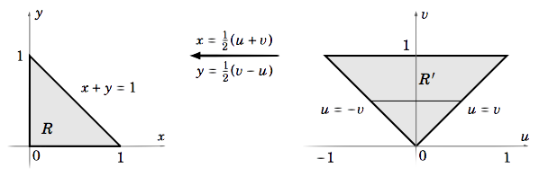
First, note that evaluating this double integral without using substitution is probably impossible, at least in a closed form. By looking at the numerator and denominator of the exponent of \(e\), we will try the substitution \(u = x − y \text{ and }v = x + y\). To use the change of variables Formula \ref{Eq3.19}, we need to write both \(x \text{ and }y\) in terms of \(u \text{ and }v\). So solving for \(x \text{ and }y\) gives \(x = \dfrac{1}{2} (u + v) \text{ and }y = \dfrac{1}{ 2} (v − u)\). In Figure \(\PageIndex{1}\) below, we see how the mapping \(x = x(u,v) = \dfrac{1}{ 2} (u+v), y = y(u,v) = \dfrac{1}{ 2} (v− u)\) maps the region \(R′\) onto \(R\) in a one-to-one manner.

Figure \(\PageIndex{1}\): The regions \(R \text{ and }R\)

Now we see that

\[\nonumber J(u,v) = \begin{vmatrix} \dfrac{∂x}{∂u} & \dfrac{∂x}{∂v} \\[4pt] \dfrac{∂y}{∂u} & \dfrac{∂y}{∂v} \\[4pt] \end{vmatrix} = \begin{vmatrix} \dfrac{1}{2} & \dfrac{1}{2} \\[4pt] -\dfrac{1}{2} & \dfrac{1}{2} \\[4pt] \end{vmatrix} = \dfrac{1}{2} \Rightarrow \lvert J(u,v) \rvert = \left\lvert \dfrac{1}{2} \right\rvert=\dfrac{1}{2} \]

so using horizontal slices in \(R'\), we have

\[\nonumber \begin{align} \iint\limits_R e^{\dfrac{x-y}{x+y}}\,dA &= \iint\limits_{R'}f (x(u,v), y(u,v))|J(u,v)|d A \\[4pt] \nonumber &=\int_0^1 \int_{-v}^v e^{u/v}\dfrac{1}{2}\,du\,dv \\[4pt] \nonumber &= \int_0^1 \left ( \dfrac{v}{2}e^{u/v} \big |_{u=-v}^{u=v} \right ) dv \\[4pt] \nonumber &=\int_0^1 \dfrac{v}{2}(e-e^1)dv \\[4pt] \nonumber &=\dfrac{v^2}{4}(e-e^1)\big |_0^1 = \dfrac{1}{4} \left ( e-\dfrac{1}{e} \right ) = \dfrac{e^2-1}{4e} \end{align}\]

The change of variables formula can be used to evaluate double integrals in polar coordinates. Letting

\[ x = x(r,θ) = r \cos{θ} \text{ and }y = y(r,θ) = r \sin{θ} , \]

we have

\[ J(u,v) = \begin{vmatrix} \dfrac{∂x}{∂r} & \dfrac{∂x}{∂θ} \\[4pt] \dfrac{∂y}{∂r} & \dfrac{∂y}{∂θ} \\[4pt] \end{vmatrix} = \begin{vmatrix} \cos{θ} & -r \sin{θ} \\[4pt] \sin{θ} & r\cos{θ} \end{vmatrix} = r \cos^2{ θ} + r \sin^2 {θ} = r \Rightarrow |J(u,v)| = |r| = r \]

so we have the following formula:

Double Integral in Polar Coordinates

\[\iint\limits_R f (x, y)\,dx\, d y = \iint\limits_{R'}f (r \cos{θ}, r \sin{θ}) r\, dr\, dθ \label{Eq3.24}\]

where the mapping \(x = r \cos{θ}, y = r \sin{θ}\) maps the region \(R′\) in the \(rθ\)-plane onto the region \(R\) in the \(x y\)-plane in a one-to-one manner.

Example \(\PageIndex{2}\): Volume of Paraboloid

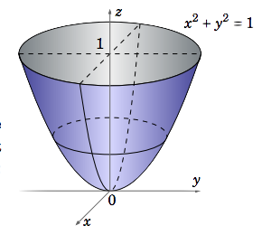
Find the volume \(V\) inside the paraboloid \(z = x^ 2 + y^ 2 \text{ for }0 ≤ z ≤ 1\)

Solution

Using vertical slices, we see that

\[\nonumber V= \iint\limits_R (1− z)d A = \iint\limits_R ( 1−(x^2 + y^ 2)) d A \]

Figure \(\PageIndex{2}\): \(z = x^ 2 + y^ 2\)

where \(R = {(x, y) : x^ 2 + y^ 2 ≤ 1}\) is the unit disk in \(\mathbb{R}^2\) (see Figure \(\PageIndex{2}\)). In polar coordinates \((r,θ)\) we know that \(x^ 2+ y^ 2 = r^ 2\) and that the unit disk \(R\) is the set \(R ′ = {(r,θ) : 0 ≤ r ≤ 1,0 ≤ θ ≤ 2\pi}\). Thus,

\[\nonumber \begin{align} V &= \int_0^{2\pi} \int_0^1 (1− r^ 2 ) r\, dr\, dθ \\[4pt] \nonumber &= \int_0^{2\pi} \int_0^1 (r − r^ 3 )dr\, dθ \\[4pt] \nonumber &= \int_o^{2\pi} \left ( \dfrac{r^2}{2}-\dfrac{r^4}{4}\big |_{r=0}^{r=1} \right )\,dθ \\[4pt] \nonumber &= \int_0^{2\pi}\dfrac{1}{4}\,dθ \\[4pt] \nonumber &=\dfrac{\pi}{2} \end{align}\]

Example \(\PageIndex{3}\): Volume of Cone

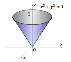
Find the volume \(V\) inside the cone \(z = \sqrt{ x^ 2 + y^ 2}\text{ for }0 ≤ z ≤ 1\).

Solution

Using vertical slices, we see that

\[\nonumber V= \iint\limits_R (1− z)d A = \iint\limits_R \left ( 1−\sqrt{x^2 + y^ 2}\right ) d A\]

Figure \(\PageIndex{3}\): \(z = \sqrt{ x^ 2 + y^ 2}\)

where \(R = {(x, y) : x^ 2 + y^ 2 ≤ 1}\) is the unit disk in \(\mathbb{R}^2\) (see Figure \(\PageIndex{3}\)). In polar coordinates \((r,θ)\) we know that \(\sqrt{x^ 2 + y^ 2 = r}\) and that the unit disk \(R\) is the set \(R ′ = {(r,θ) : 0 ≤ r ≤ 1,0 ≤ θ ≤ 2\pi}\). Thus,

\[\nonumber \begin{align} V &= \int_0^{2\pi}\int_0^1(1− r) r\, dr\, dθ \\[4pt] \nonumber &=\int_0^{2\pi}\int_0^1(r − r^ 2 )dr\, dθ \\[4pt] \nonumber &=\int_0^{2\pi} \left ( \dfrac{r^2}{2}-\dfrac{r^3}{3}\big |_{r=0}^{r=1} \right )dθ \\[4pt] \nonumber &= \int_0^{2\pi} \dfrac{1}{6}dθ \\[4pt] \nonumber &=\dfrac{\pi}{3} \end{align} \]

In a similar fashion, it can be shown (see Exercises 5-6) that triple integrals in cylindrical and spherical coordinates take the following forms:

Triple Integral in Cylindrical Coordinates

\[\iiint\limits_S f (x, y, z)dx\, d y\, dz =\iiint\limits_{S'} (r \cos{θ}, r \sin{θ}, z) r\, dr\, dθ\, dz \label{Eq3.25}\]

where the mapping \(x = r \cos{θ}, y = r \sin{θ}, z = z\) maps the solid \(S ′\) in \(rθz\)-space onto the solid \(S \text{ in }x yz\)-space in a one-to-one manner.

Triple Integral in Spherical Coordinates

\[\iiint\limits_S f (x, y, z)dx\, d y\, dz = \iiint\limits_{S'}f (ρ \sin{φ} \cos{θ},ρ \sin{φ} \sin{θ},ρ \cos{φ})ρ^2 \sin{φ}dρ\, dφ\,dθ \label{Eq3.26}\]

where the mapping \(x = ρ \sin{φ} \cos{θ}, y = ρ \sin{φ} \sin{θ}, z = ρ \cos{φ} \)maps the solid \(S ′\) in \(ρφθ\)- space onto the solid \(S\) in \(x yz\)-space in a one-to-one manner.

Example \(\PageIndex{4}\)

For \(a > 0\), find the volume \(V\) inside the sphere \(S = x^ 2 + y^ 2 + z^ 2 = a^ 2\).

Solution

We see that \(S\) is the set \(ρ = a\) in spherical coordinates, so

\[\nonumber \begin{align} V&=\iiint\limits_S 1dV = \int_0^{2\pi}\int_0^{\pi}\int_0^a 1ρ^2 \sin{φ}dρ\, dφ\,dθ \\[4pt] \nonumber &= \int_0^{2\pi}\int_0^{\pi} \left ( \dfrac{ρ^ 3}{3}\big |_{ρ=0}^{ρ=a} \right ) \sin{φ}dφ\,dθ = \int_0^{2\pi}\int_0^{\pi}\dfrac{a^3}{3}\sin{φ}dφ\,dθ \\[4pt] \nonumber &=\int_0^{2\pi} \left (-\dfrac{a^3}{3}\cos{φ}\big |_{φ=0}^{ φ=π} \right )dθ = \int_0^{2\pi} \dfrac{2a^3}{3}dθ = \dfrac{4\pi a^3}{3}\end{align}\]