
5.1: Graphs
- Page ID
- 95654

\( \newcommand{\vecs}[1]{\overset { \scriptstyle \rightharpoonup} {\mathbf{#1}} } \)
\( \newcommand{\vecd}[1]{\overset{-\!-\!\rightharpoonup}{\vphantom{a}\smash {#1}}} \)
\( \newcommand{\dsum}{\displaystyle\sum\limits} \)
\( \newcommand{\dint}{\displaystyle\int\limits} \)
\( \newcommand{\dlim}{\displaystyle\lim\limits} \)
\( \newcommand{\id}{\mathrm{id}}\) \( \newcommand{\Span}{\mathrm{span}}\)
( \newcommand{\kernel}{\mathrm{null}\,}\) \( \newcommand{\range}{\mathrm{range}\,}\)
\( \newcommand{\RealPart}{\mathrm{Re}}\) \( \newcommand{\ImaginaryPart}{\mathrm{Im}}\)
\( \newcommand{\Argument}{\mathrm{Arg}}\) \( \newcommand{\norm}[1]{\| #1 \|}\)
\( \newcommand{\inner}[2]{\langle #1, #2 \rangle}\)
\( \newcommand{\Span}{\mathrm{span}}\)
\( \newcommand{\id}{\mathrm{id}}\)
\( \newcommand{\Span}{\mathrm{span}}\)
\( \newcommand{\kernel}{\mathrm{null}\,}\)
\( \newcommand{\range}{\mathrm{range}\,}\)
\( \newcommand{\RealPart}{\mathrm{Re}}\)
\( \newcommand{\ImaginaryPart}{\mathrm{Im}}\)
\( \newcommand{\Argument}{\mathrm{Arg}}\)
\( \newcommand{\norm}[1]{\| #1 \|}\)
\( \newcommand{\inner}[2]{\langle #1, #2 \rangle}\)
\( \newcommand{\Span}{\mathrm{span}}\) \( \newcommand{\AA}{\unicode[.8,0]{x212B}}\)
\( \newcommand{\vectorA}[1]{\vec{#1}} % arrow\)
\( \newcommand{\vectorAt}[1]{\vec{\text{#1}}} % arrow\)
\( \newcommand{\vectorB}[1]{\overset { \scriptstyle \rightharpoonup} {\mathbf{#1}} } \)
\( \newcommand{\vectorC}[1]{\textbf{#1}} \)
\( \newcommand{\vectorD}[1]{\overrightarrow{#1}} \)
\( \newcommand{\vectorDt}[1]{\overrightarrow{\text{#1}}} \)
\( \newcommand{\vectE}[1]{\overset{-\!-\!\rightharpoonup}{\vphantom{a}\smash{\mathbf {#1}}}} \)
\( \newcommand{\vecs}[1]{\overset { \scriptstyle \rightharpoonup} {\mathbf{#1}} } \)
\(\newcommand{\longvect}{\overrightarrow}\)
\( \newcommand{\vecd}[1]{\overset{-\!-\!\rightharpoonup}{\vphantom{a}\smash {#1}}} \)
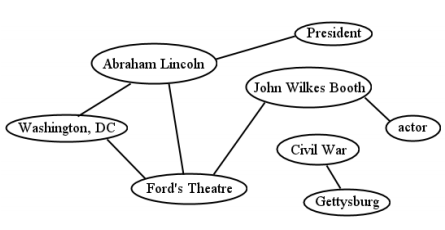
\(\newcommand{\avec}{\mathbf a}\) \(\newcommand{\bvec}{\mathbf b}\) \(\newcommand{\cvec}{\mathbf c}\) \(\newcommand{\dvec}{\mathbf d}\) \(\newcommand{\dtil}{\widetilde{\mathbf d}}\) \(\newcommand{\evec}{\mathbf e}\) \(\newcommand{\fvec}{\mathbf f}\) \(\newcommand{\nvec}{\mathbf n}\) \(\newcommand{\pvec}{\mathbf p}\) \(\newcommand{\qvec}{\mathbf q}\) \(\newcommand{\svec}{\mathbf s}\) \(\newcommand{\tvec}{\mathbf t}\) \(\newcommand{\uvec}{\mathbf u}\) \(\newcommand{\vvec}{\mathbf v}\) \(\newcommand{\wvec}{\mathbf w}\) \(\newcommand{\xvec}{\mathbf x}\) \(\newcommand{\yvec}{\mathbf y}\) \(\newcommand{\zvec}{\mathbf z}\) \(\newcommand{\rvec}{\mathbf r}\) \(\newcommand{\mvec}{\mathbf m}\) \(\newcommand{\zerovec}{\mathbf 0}\) \(\newcommand{\onevec}{\mathbf 1}\) \(\newcommand{\real}{\mathbb R}\) \(\newcommand{\twovec}[2]{\left[\begin{array}{r}#1 \\ #2 \end{array}\right]}\) \(\newcommand{\ctwovec}[2]{\left[\begin{array}{c}#1 \\ #2 \end{array}\right]}\) \(\newcommand{\threevec}[3]{\left[\begin{array}{r}#1 \\ #2 \\ #3 \end{array}\right]}\) \(\newcommand{\cthreevec}[3]{\left[\begin{array}{c}#1 \\ #2 \\ #3 \end{array}\right]}\) \(\newcommand{\fourvec}[4]{\left[\begin{array}{r}#1 \\ #2 \\ #3 \\ #4 \end{array}\right]}\) \(\newcommand{\cfourvec}[4]{\left[\begin{array}{c}#1 \\ #2 \\ #3 \\ #4 \end{array}\right]}\) \(\newcommand{\fivevec}[5]{\left[\begin{array}{r}#1 \\ #2 \\ #3 \\ #4 \\ #5 \\ \end{array}\right]}\) \(\newcommand{\cfivevec}[5]{\left[\begin{array}{c}#1 \\ #2 \\ #3 \\ #4 \\ #5 \\ \end{array}\right]}\) \(\newcommand{\mattwo}[4]{\left[\begin{array}{rr}#1 \amp #2 \\ #3 \amp #4 \\ \end{array}\right]}\) \(\newcommand{\laspan}[1]{\text{Span}\{#1\}}\) \(\newcommand{\bcal}{\cal B}\) \(\newcommand{\ccal}{\cal C}\) \(\newcommand{\scal}{\cal S}\) \(\newcommand{\wcal}{\cal W}\) \(\newcommand{\ecal}{\cal E}\) \(\newcommand{\coords}[2]{\left\{#1\right\}_{#2}}\) \(\newcommand{\gray}[1]{\color{gray}{#1}}\) \(\newcommand{\lgray}[1]{\color{lightgray}{#1}}\) \(\newcommand{\rank}{\operatorname{rank}}\) \(\newcommand{\row}{\text{Row}}\) \(\newcommand{\col}{\text{Col}}\) \(\renewcommand{\row}{\text{Row}}\) \(\newcommand{\nul}{\text{Nul}}\) \(\newcommand{\var}{\text{Var}}\) \(\newcommand{\corr}{\text{corr}}\) \(\newcommand{\len}[1]{\left|#1\right|}\) \(\newcommand{\bbar}{\overline{\bvec}}\) \(\newcommand{\bhat}{\widehat{\bvec}}\) \(\newcommand{\bperp}{\bvec^\perp}\) \(\newcommand{\xhat}{\widehat{\xvec}}\) \(\newcommand{\vhat}{\widehat{\vvec}}\) \(\newcommand{\uhat}{\widehat{\uvec}}\) \(\newcommand{\what}{\widehat{\wvec}}\) \(\newcommand{\Sighat}{\widehat{\Sigma}}\) \(\newcommand{\lt}{<}\) \(\newcommand{\gt}{>}\) \(\newcommand{\amp}{&}\) \(\definecolor{fillinmathshade}{gray}{0.9}\)In many ways, the most elegant, simple, and powerful way of representing knowledge is by means of a graph. A graph is composed of a bunch of little bits of data, each of which may (or may not) be attached to each of the others. An example is in Figure \(\PageIndex{1}\) . Each of the labeled ovals is called a vertex (plural: vertices), and the lines between them are called edges. Each vertex does, or does not, contain an edge connecting it to each other vertex. One could imagine each of the vertices containing various descriptive attributes — perhaps the John Wilkes Booth oval would have information about Booth’s birthdate, and Washington, DC information about its longitude, latitude, and population — but these are typically not shown on the diagram. All that really matters, graph-wise, is what vertices it contains, and which ones are joined to which others.
Cognitive psychologists, who study the internal mental processes of the mind, have long identified this sort of structure as the principal way that people mentally store and work with information. After all, if you step back a moment and ask “what is the ‘stuff’ that’s in my memory?" a reasonable answer is “well I know about a bunch of things, and the properties of those things, and the relationships between those things." If the “things" are vertices, and the “properties" are attributes of those vertices, and the “relationships" are the edges, we have precisely the structure of a graph. Psychologists have given this another name: a semantic network. It is thought that the myriad of concepts you have committed to memory — Abraham Lincoln, and bar of soap, and my fall schedule, and perhaps millions of others — are all associated in your mind in a vast semantic network that links the related concepts together. When your mind recalls information, or deduces facts, or even drifts randomly in idle moments, it’s essentially traversing this graph along the various edges that exist between vertices.
That’s deep. But you don’t have to go near that deep to see the appearance of graph structures all throughout computer science. What’s MapQuest, if not a giant graph where the vertices are travelable locations and the edges are routes between them? What’s Facebook, if not a giant graph where the vertices are people and the edges are friendships? What’s the World Wide Web, if not a giant graph where the vertices are pages and the edges are hyperlinks? What’s the Internet, if not a giant graph where the vertices are computers or routers and the edges are communication links between them? This simple scheme of linked vertices is powerful enough to accommodate a whole host of applications, which is why it’s worth studying.
Graph terms
The study of graphs brings with it a whole bevy of new terms which are important to use precisely:
vertex. Every graph contains zero or more vertices.1 (These are also sometimes called nodes, concepts, or objects.)
edge. Every graph contains zero or more edges. (These are also sometimes called links, connections, associations, or relationships.) Each edge connects exactly two vertices, unless the edge connects a vertex to itself, which is possible, believe it or not. An edge that connects a vertex to itself is called a loop.
path. A path is a sequence of consecutive edges that takes you from one vertex to the other. In Figure \(\PageIndex{1}\) , there is a path between Washington, DC and John Wilkes Booth (by means of Ford’s Theatre) even though there is no direct edge between the two. By contrast, no path exists between President and Civil War. Don’t confuse the two terms edge and path: the former is a single link between two nodes, while the second can be a whole step-by-step traversal. (A single edge does count as a path, though.)
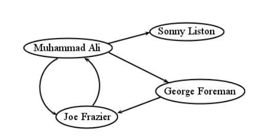
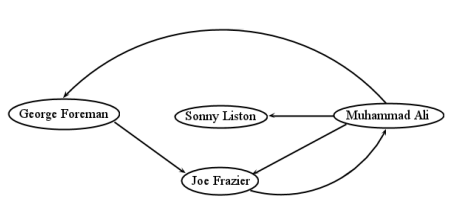
directed/undirected. In some graphs, relationships between nodes are inherently bidirectional: if \(A\) is linked to \(B\), then \(B\) is linked to \(A\), and it doesn’t make sense otherwise. Think of Facebook: friendship always goes both ways. This kind of graph is called an undirected graph, and like the Abraham Lincoln example in Figure \(\PageIndex{1}\) , the edges are shown as straight lines. In other situations, an edge from \(A\) to \(B\) doesn’t necessarily imply one in the reverse direction as well. In the World Wide Web, for instance, just because webpage \(A\) has a link on it to webpage \(B\) doesn’t mean the reverse is true (it usually isn’t). In this kind of directed graph, we draw arrowheads on the lines to indicate which way the link goes. An example is Figure \(\PageIndex{2}\) : the vertices represent famous boxers, and the directed edges indicate which boxer defeated which other(s). It is possible for a pair of vertices to have edges in both directions — Muhammad Ali and Joe Frazier each defeated the other (in separate bouts, of course) — but this is not the norm, and certainly not the rule, with a directed graph.
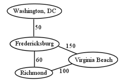
weighted. Some graphs, in addition to merely containing the presence (or absence) of an edge between each pair of vertices, also have a number on each edge, called the edge’s weight. Depending on the graph, this can indicate the distance, or cost, between vertices. An example is in Figure \(\PageIndex{3}\) : in true MapQuest fashion, this graph contains locations, and the mileage between them. A graph can be both directed and weighted, by the way. If a pair of vertices in such a graph is attached “both ways," then each of the two edges will have its own weight.
adjacent. If two vertices have an edge between them, they are said to be adjacent.
connected. The word connected has two meanings: it applies both to pairs of vertices and to entire graphs.
We say that two vertices are connected if there is at least one path between them. Each vertex is therefore “reachable" from the other. In Figure \(\PageIndex{1}\) , President and actor are connected, but Ford’s Theatre and Civil War are not.
“Connected" is also used to describe entire graphs, if every node can be reached from all others. It’s easy to see that Figure \(\PageIndex{3}\) is a connected graph, whereas Figure \(\PageIndex{1}\) is not (because Civil War and Gettysburg are isolated from the other nodes). It’s not always trivial to determine whether a graph is connected, however: imagine a tangled morass of a million vertices, with ten million edges, and having to figure out whether or not every vertex is reachable from every other. (And if that seems unrealistically large, consider Facebook, which has over a billion nodes.)
degree. A vertex’s degree is simply the number of edges that connect to it. Virginia Beach has degree 2, and Fredericksburg 3. In the case of a directed graph, we sometimes distinguish between the number of incoming arrows a vertex has (called its in-degree) and the number of outgoing arrows (the out-degree). Muhammad Ali had a higher out-degree (3) than in-degree (1) since he won most of the time.
cycle. A cycle is a path that begins and ends at the same vertex.2 In Figure \(\PageIndex{3}\) , Richmond–to–Virginia Beach–to–Fredericksburg–to–Richmond is a cycle. Any loop is a cycle all by itself. For directed graphs, the entire loop must comprise edges in the “forward" direction: no fair going backwards. In Figure \(\PageIndex{2}\) , Frazier–to–Ali–to–Foreman–to–Frazier is a cycle, as is the simpler Ali–to–Frazier–to–Ali.
DAG (directed, acyclic graph). One common use of graphs is to represent flows of dependencies, for instance the prerequisites that different college courses have for one another. Another example is project management workflows: the tasks needed to complete a project become vertices, and then the dependencies they have on one another become edges. The graph in Figure \(\PageIndex{4}\) shows the steps in making a batch of brownies, and how these steps depend on each other. The eggs have to be cracked before the ingredients can be mixed, and the oven has to be preheated before baking, but the pan can be greased any old time, provided that it’s done before pouring the brown goop into it.
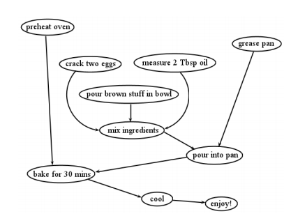
A graph of dependencies like this must be both directed and acyclic, or it wouldn’t make sense. Directed, of course, means that task X can require task Y to be completed before it, without the reverse also being true. If they both depended on each other, we’d have an infinite loop, and no brownies could ever get baked! Acyclic means that no kind of cycle can exist in the graph, even one that goes through multiple vertices. Such a cycle would again result in an infinite loop, making the project hopeless. Imagine if there were an arrow from bake for 30 mins back to grease pan in Figure \(\PageIndex{4}\) . Then, we’d have to grease the pan before pouring the goop into it, and we’d have to pour the goop before baking, but we’d also have to bake before greasing the pan! We’d be stuck right off the bat: there’d be no way to complete any of those tasks since they’d all indirectly depend on each other. A graph that is both directed and acyclic (and therefore free of these problems) is sometimes called a DAG for short.
Spatial positioning
One important thing to understand about graphs is which aspects of a diagram are relevant. Specifically, the spatial positioning of the vertices doesn’t matter. In Figure \(\PageIndex{2}\) we drew Muhammad Ali in the mid-upper left, and Sonny Liston in the extreme upper right. But this was an arbitrary choice, and irrelevant. More specifically, this isn’t part of the information the diagram claims to represent. We could have positioned the vertices differently, as in Figure \(\PageIndex{5}\), and had the same graph. In both diagrams, there are the same vertices, and the same edges between them (check me). Therefore, these are mathematically the same graph.
This might not seem surprising for the prize fighter graph, but for graphs like the MapQuest graph, which actually represent physical locations, it can seem jarring. In Figure \(\PageIndex{3}\) we could have drawn Richmond north of Fredericksburg, and Virginia Beach on the far west side of the diagram, and still had the same graph, provided that all the nodes and links were the same. Just remember that the spatial positioning is designed for human convenience, and isn’t part of the mathematical information. It’s similar to how there’s no order to the elements of a set, even though when we specify a set extensionally, we have to list them in some order to avoid writing all the element names on top of each other. On a graph diagram, we have to draw each vertex somewhere, but where we put it is simply aesthetic.
We seem to have strayed far afield from sets with all this graph stuff. But actually, there are some important connections to be made to those original concepts. Recall the wizards set \(A\) from chapter that we extended to contain { Harry, Ron, Hermione, Neville }. Now consider the following endorelation on \(A\):
(Harry, Ron)
(Ron, Harry)
(Ron, Hermione)
(Ron, Neville)
(Hermione, Hermione)
(Neville, Harry)
This relation, and all it contains, is represented faithfully by the graph in Figure \(\PageIndex{6}\) . The elements of \(A\) are the vertices of course, and each ordered pair of the relation is reflected in an edge of the graph. Can you see how exactly the same information is represented by both forms?
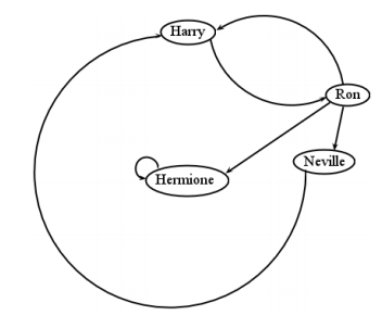
Figure \(\PageIndex{6}\) is a directed graph, of course. What if it were an undirected graph? The answer is that the corresponding relation would be symmetric. An undirected graph implies that if there’s an edge between two vertices, it goes “both ways." This is really identical to saying a relation is symmetric: if an \((x,y)\) is in the relation, then the corresponding \((y,x)\) must also be. An example is Figure \(\PageIndex{7}\) , which depicts the following symmetric relation:
(Harry, Ron)
(Ron, Harry)
(Ron, Hermione)
(Hermione, Ron)
(Harry, Harry)
(Neville, Neville)
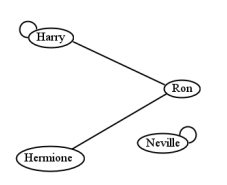
Notice how the loops (edges from a node back to itself) in these diagrams represent ordered pairs in which both elements are the same.
Another connection between graphs and sets has to do with partitions. Figure \(\PageIndex{7}\) was not a connected graph: Neville couldn’t be reached from any of the other nodes. Now consider: isn’t a graph like this similar in some ways to a partition of \(A\) — namely, this one?
{ Harry, Ron, Hermione } and { Neville }.
We’ve simply partitioned the elements of \(A\) into the groups that are connected. If you remove the edge between Harry and Ron in that graph, you have:
{ Harry }, { Ron, Hermione }, and { Neville }.
Then add one between Hermione and Neville, and now you have:
{ Harry } and { Ron, Hermione, Neville }.
In other words, the “connectedness" of a graph can be represented precisely as a partition of the set of vertices. Each connected subset is in its own group, and every vertex is in one and only one group: therefore, these isolated groups are mutually exclusive and collectively exhaustive. Cool.
Graph traversal
If you had a long list — perhaps of phone numbers, names, or purchase orders — and you needed to go through and do something to each element of the list — dial all the numbers, scan the list for a certain name, add up all the orders — it’d be pretty obvious how to do it. You just start at the top and work your way down. It might be tedious, but it’s not confusing.
Iterating through the elements like this is called traversing the data structure. You want to make sure you encounter each element once (and only once) so you can do whatever needs to be done with it. It’s clear how to traverse a list. But how to traverse a graph? There is no obvious “first" or “last" node, and each one is linked to potentially many others. And as we’ve seen, the vertices might not even be fully connected, so a traversal path through all the nodes might not even exist.
There are two different ways of traversing a graph: breadth-first, and depth-first. They provide different ways of exploring the nodes, and as a side effect, each is able to discover whether the graph is connected or not. Let’s look at each in turn.
Breadth-first traversal
With breadth-first traversal, we begin at a starting vertex (it doesn’t matter which one) and explore the graph cautiously and delicately. We probe equally deep in all directions, making sure we’ve looked a little ways down each possible path before exploring each of those paths a little further.
To do this, we use a very simple data structure called a queue. A queue is simply a list of nodes that are waiting in line. (In Britain, I’m told, instead of saying “line up" at the sandwich shop, they say “queue up.") When we enter a node into the queue at the tail end, we call it enqueueing the node, and when we remove one from the front, we call it dequeueing the node. The nodes in the middle patiently wait their turn to be dealt with, getting closer to the front every time the front node is dequeued.
An example of this data structure in action is shown in Table \(\PageIndex{1}\) . Note carefully that we always insert nodes at one end (on the right) and remove them from the other end (the left). This means that the first item to be enqueued (in this case, the triangle) will be the first to be dequeued. “Calls will be answered in the order they were received." This fact has given rise to another name for a queue: a “FIFO," which stands for “first-in-first-out."
| Start with an empty queue: | \(|\) |
| Enqueue a triangle, and we have: | \(|\triangle\) |
| Enqueue a star, and we have: | \(|\triangle \bigstar\) |
| Enqueue a heart, and we have: | \(|\triangle \bigstar \heartsuit\) |
| Dequeue the triangle, and we have: | \(|\bigstar \heartsuit\) |
| Enqueue a club, and we have: | \(|\bigstar \heartsuit \clubsuit\) |
| Dequeue the star, and we have: | \(|\heartsuit \clubsuit\) |
| Dequeue the heart, and we have: | \(|\clubsuit\) |
| Dequeue the club. We’re empty again: | \(|\) |
Now here’s how we use a queue to traverse a graph breadth-first. We’re going to start at a particular node, and put all of its adjacent nodes into a queue. This makes them all safely “wait in line" until we get around to exploring them. Then, we repeatedly take the first node in line, do whatever we need to do with it, and then put all of its adjacent nodes in line. We keep doing this until the queue is empty.
Now it might have occurred to you that we can run into trouble if we encounter the same node multiple times while we’re traversing. This can happen if the graph has a cycle: there will be more than one path to reach some nodes, and we could get stuck in an infinite loop if we’re not careful. For this reason, we introduce the concept of marking nodes. This is kind of like leaving a trail of breadcrumbs: if we’re ever about to explore a node, but find out it’s marked, then we know we’ve already been there, and it’s pointless to search it again.
So there are two things we’re going to do to nodes as we search:
-
To mark a node means to remember that we’ve already encountered it in the process of our search.
-
To visit a node means to actually do whatever it is we need to do to the node (call the phone number, examine its name for a pattern match, add the number to our total, whatever.)
Now then. Breadth-first traversal (BFT) is an algorithm, which is just a step-by-step, reliable procedure that’s guaranteed to produce a result. In this case, it’s guaranteed to visit every node in the graph that’s reachable from the starting node, and not get stuck in any infinite loops in the process. Here it is:
-
Choose a starting node.
-
Mark it and enqueue it on an empty queue.
-
While the queue is not empty, do these steps:
-
Dequeue the front node of the queue.
-
Visit it.
-
Mark and enqueue all of its unmarked adjacent nodes (in any order).
-
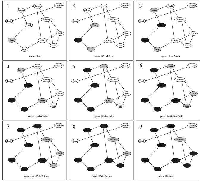
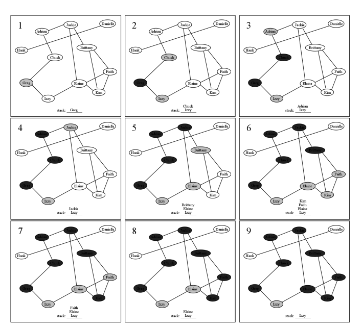
Let’s run this algorithm in action on a set of Facebook users. Figure \(\PageIndex{1}\) depicts eleven users, and the friendships between them. First, we choose Greg as the starting node (not for any particular reason, just that we have to start somewhere). We mark him (in grey on the diagram) and put him in the queue (the queue contents are listed at the bottom of each frame, with the front of the queue on the left). Then, we begin our loop. When we take Greg off the queue, we visit him (which means we “do whatever we need to do to Greg") and then mark and enqueue his adjacent nodes Chuck and Izzy. It does not matter which order we put them into the queue, just as it did not matter what node we started with. In pane 3, Chuck has been dequeued, visited, and his adjacent nodes put on the queue. Only one node gets enqueued here — Adrian — because obviously Greg has already been marked (and even visited, no less) and this marking allows us to be smart and not re-enqueue him.
It’s at this point that the “breadth-first" feature becomes apparent. We’ve just finished with Chuck, but instead of exploring Adrian next, we resume with Izzy. This is because she has been waiting patiently on the queue, and her turn has come up. So we lay Adrian aside (in the queue, of course) and visit Izzy, enqueueing her neighbor Elaine in the process. Then, we go back to Adrian. The process continues, in “one step on the top path, one step on the bottom path" fashion, until our two exploration paths actually meet each other on the back end. Visiting Jackie causes us to enqueue Brittany, and then when we take Kim off the queue, we do not re-enqueue Brittany because she has been marked and so we know she’s already being taken care of.
For space considerations, Figure \(\PageIndex{1}\) leaves off at this point, but of course we would continue visiting nodes in the queue until the queue was empty. As you can see, Hank and Danielle will not be visited at all in this process: this is because apparently nobody they know knows anybody in the Greg crowd, and so there’s no way to reach them from Greg. This is what I meant earlier by saying that as a side effect, the BFT algorithm tells us whether the graph is connected or not. All we have to do is start somewhere, run BFT, and then see whether any nodes have not been marked and visited. If there are any, we can continue with another starting point, and then repeat the process.
Depth-first traversal (DFT)
With depth-first traversal, we explore the graph boldly and recklessly. We choose the first direction we see, and plunge down it all the way to its depths, before reluctantly backing out and trying the other paths from the start.
The algorithm is almost identical to BFT, except that instead of a queue, we use a stack. A stack is the same as a queue except that instead of putting elements on one end and taking them off the other, you add and remove to the same end. This “end" is called the top of the stack. When we add an element to this end, we say we push it on the stack, and when we remove the top element, we say we pop it off.
| Start with an empty stack: | \(\underline{\quad}\) |
| Push a triangle, and we have: | \(\underline{\triangle}\) |
| Push a star, and we have: | \(\bigstar\)\(\underline{\triangle}\) |
| Push a heart, and we have: | \(\heartsuit\)\(\bigstar\)\(\underline{\triangle}\) |
| Pop the heart, and we have: | \(\bigstar\)\(\underline{\triangle}\) |
| Push a club, and we have: | \(\clubsuit\)\(\bigstar\)\(\underline{\triangle}\) |
| Pop the club, and we have: | \(\bigstar\)\(\underline{\triangle}\) |
| Pop the star, and we have: | \(\underline{\triangle}\) |
| Pop the triangle. We’re empty again: | \(\underline{\quad}\) |
You can think of a stack as...well, a stack, whether of books or cafeteria trays or anything else. You can’t get anything out of the middle of a stack, but you can take items off and put more items on. Table\(\PageIndex{2}\) has an example. The first item pushed is always the last one to be popped, and the most recent one pushed is always ready to be popped back off, and so a stack is also sometimes called a “LIFO" (last-in-first-out.)
The depth-first traversal algorithm itself looks like déjà vu all over again. All you do is replace “queue" with “stack":
-
Choose a starting node.
-
Mark it and push it on an empty stack.
-
While the stack is not empty, do these steps:
-
Pop the top node off the stack.
-
Visit it.
-
Mark and push all of its unmarked adjacent nodes (in any order).
-
The algorithm in action is shown in Figure \(\PageIndex{9}\). The stack really made a difference! Instead of alternately exploring Chuck’s and Izzy’s paths, it bullheadedly darts down Chuck’s path as far as it can go, all the way to hitting Izzy’s back door. Only then does it back out and visit Izzy. This is because the stack always pops off what it just pushed on, whereas whatever got pushed first has to wait until everything else is done before it gets its chance. That first couple of pushes was critical: if we had pushed Chuck before Izzy at the very beginning, then we would have explored Izzy’s entire world before arriving at Chuck’s back door, instead of the other way around. As it is, Izzy got put on the bottom, and so she stayed on the bottom, which is inevitable with a stack.
DFT identifies disconnected graphs in the same way as BFT, and it similarly avoids getting stuck in infinite loops when it encounters cycles. The only difference is the order in which it visits the nodes.
Finding the shortest path
We’ll look at two other important algorithms that involve graphs, specifically weighted graphs. The first one is called Dijkstra’s shortest-path algorithm. This is a procedure for finding the shortest path between two nodes, if one exists. It was invented in 1956 by the legendary computer science pioneer Edsger Dijkstra, and is widely used today by, among other things, network routing protocols.
Consider Figure \(\PageIndex{10}\) , a simplified map of France circa November 1944. Fresh U.S. troops are arriving by ship at the port town of Bordeaux, and need to reach Strasbourg as quickly as possible to assist the Allies in pushing Nazi squadrons back into Germany. The vertices of this graph are French cities, and the edge weights represent marching distances in kilometers. Although D-Day was successful, the outcome of the War may depend on how quickly these reinforcements can reach the front.
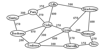
The question, obviously, is which path the troops should take so as to reach Strasbourg the soonest. With a graph this small, you might be able to eyeball it. (Try it!) But Dijksta’s algorithm systematically considers every possible path, and is guaranteed to find the one with the shortest total distance.
The way it works is to assign each node a tentative lowest distance, along with a tentative path from the start node to it. Then, if the algorithm encounters a different path to the same node as it progresses, it updates this tentative distance with the new, lower distance, and replaces the “best path to it" with the new one. Dijkstra’s algorithm finds the shortest distance from the start node to the end node, but as a bonus, it actually finds the shortest distance from the start node to every node as it goes. Thus you are left with the best possible path from your start node to every other node in the graph.
Here’s the algorithm in full:
-
Choose a starting node and an ending node.
-
Mark the tentative distance for the starting nodes as 0, and all other nodes as \(\infty\).
-
While there are still unvisited nodes, do these steps:
-
[choose] Identify the unvisited node with the smallest tentative distance. (If this is \(\infty\), then we’re done. All other nodes are unreachable.) Call this node the “current node."
-
For each unvisited neighbor of the current node, do these steps:
-
Compute the sum of the current node’s tentative distance and the distance from the current node to its neighbor.
-
Compare this total to the neighbor’s current tentative distance. If it’s less than the current tentative distance, update the tentative distance with this new value, and mark an arrow on the path from the current node to the neighbor (erasing any other arrow to the neighbor.)
-
Mark the current node as visited. (Its distance and best path are now fixed.)
-
-
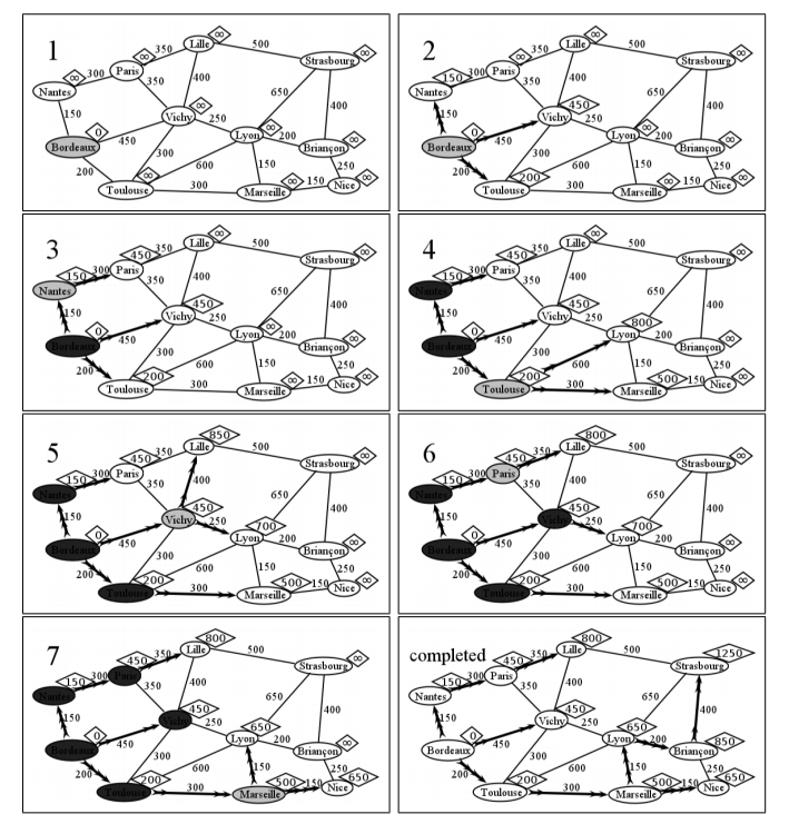
Don’t worry, this isn’t as hard as it sounds. But you do have to have your wits about you and carefully update all the numbers. Let’s see it in action for WWII France. In the first frame of Figure \(\PageIndex{11}\) , we’ve marked each node with a diamond containing the tentative shortest distance to it from Bordeaux. This is 0 for Bordeaux itself (since it’s 0 kilometers away from itself, duh), and infinity for all the others, since we haven’t explored anything yet, and we want to start off as pessimistic as possible. We’ll update this distances to lower values as we find paths to them.
We start with Bordeaux as the “current node," marked in grey. In frame 2, we update the best-possible-path and the distance-of-that-path for each of Bordeaux’s neighbors. Nantes, we discover, is no longer “infinity away," but a mere 150 km away, since there is a direct path to it from Bordeaux. Vichy and Toulouse are similarly updated. Note the heavy arrowed lines on the diagram, showing the best path (so far) to each of these cities from Bordeaux.
Step 3.1 tells us to choose the node with the lowest tentative distance as the next current node. So for frame 3, Nantes fits the bill with a (tentative) distance of 150 km. It has only one unmarked neighbor, Paris, which we update with 450 km. Why 450? Because it took us 150 to get from the start to Nantes, and another 300 from Nantes to Paris. After updating Paris, Nantes is now set in stone — we know we’ll never encounter a better route to it than from Bordeaux directly.
Frame 4 is our first time encountering a node that already has a non-infinite tentative distance. In this case, we don’t further update it, because our new opportunity (Bordeaux–to–Toulouse–to–Vichy) is 500 km, which is longer than going from Bordeaux to Toulouse direct. Lyon and Marseille are updated as normal.
We now have two unmarked nodes that tie for shortest tentative distance: Paris, and Vichy (450 km each). In this case, it doesn’t matter which we choose. We’ll pick Vichy for no particular reason. Frame 5 then shows some interesting activity. We do not update the path to Paris, since it would be 800 km through Vichy, whereas Paris already had a much better 450 km path. Lille is updated from infinity to 850 km, since we found our first path to it. But Lyon is the really interesting case. It already had a path — Bordeaux–to–Toulouse–to–Lyon — but that path was 800 km, and we have just found a better path: Bordeaux–to–Vichy–to–Lyon, which only costs 450 + 250 = 700. This means we remove the arrow from Toulouse to Lyon and draw a new arrow from Vichy to Lyon. Note that the arrow from Bordeaux to Toulouse doesn’t disappear, even though it was part of this apparently-not-so-great path to Lyon. That’s because the best route to Toulouse still is along that edge. Just because we wouldn’t use it to go to Lyon doesn’t mean we don’t want it if we were going simply to Toulouse.
In frame 6, we take up the other 450 node (Paris) which we temporarily neglected when we randomly chose to continue with Vichy first. When we do, we discover a better path to Lille than we had before, and so we update its distance (to 800 km) and its path (through Nantes and Paris instead of through Vichy) accordingly.
When we consider Marseille in frame 7, we find another better path: this time to Lyon. Forget that through–Vichy stuff; it turns out to be a bit faster to go through Toulouse and Marseille. In other news, we found a way to Nice.
Hopefully you get the pattern. We continue selecting the unmarked node with the lowest tentative distance, updating its neighbors’ distances and paths, then marking it “visited," until we’re done with all the nodes. The last frame shows the completed version (with all nodes colored white again so you can read them). The verdict is: our troops should go from Bordeaux through Toulouse, Marseille, Lyon, and Briançon on their way to the fighting in Strasborg, for a total of 1,250 kilometers. Who knew? All other paths are longer. Note also how in the figure, the shortest distance to every node is easily identified by looking at the heavy arrowed lines.
Finding the minimal connecting edge set
So we’ve figured out the shortest path for our troops. But our field generals might also want to do something different: establish supply lines. A supply line is a safe route over which food, fuel, and machinery can be delivered, with smooth travel and protection from ambush. Now we have military divisions stationed in each of the eleven French cities, and so the cities must all be connected to each other via secure paths. Safeguarding each mile of a supply line takes resources, though, so we want to do this in the minimal possible way. How can we get all the cities connected to each other so we can safely deliver supplies between any of them, using the least possible amount of road?
This isn’t just a military problem. The same issue came up in ancient Rome when aqueducts had to reach multiple cities. More recently, supplying neighborhoods and homes with power, or networking multiple computers with Ethernet cable, involves the same question. In all these cases, we’re not after the shortest route between two points. Instead, we’re sort of after the shortest route “between all the points." We don’t care how each pair of nodes is connected, provided that they are connected. And it’s the total length of the required connections that we want to minimize.
To find this, we’ll use Prim’s algorithm, a technique named for the somewhat obscure computer scientist Robert Prim who developed it in 1957, although it had already been discovered much earlier (1930, by the Czech mathematician Vojtech Jarnik). Prim’s algorithm turns out to be much easier to carry out than Dijkstra’s algorithm, which I find surprising, since it seems to be solving a problem that’s just as hard. But here’s all you do:
-
Choose a node, any node.
-
While not all the nodes are connected, do these steps:
-
[greedystep] Identify the node closest to the already-connected nodes, and connect it to those nodes via the shortest edge.
-
That’s it. Prim’s algorithm is an example of a greedy algorithm, which means that it always chooses the immediately obvious short-term best choice available. Non-greedy algorithms can say, “although doing X would give the highest short-term satisfaction, I can look ahead and see that choosing Y instead will lead to a better overall result in the long run." Greedy algorithms, by contrast, always gobble up what seems best at the time. That’s what Prim’s algorithm is doing in step 2.1. It looks for the non-connected node that’s immediately closest to the connected group, and adds it without a second thought. There’s no notion of “perhaps I’ll get a shorter overall edge set if I forego connecting this temptingly close node right now."
Sometimes, a greedy algorithm turns out to give an optimal result. Often it does not, and more sophisticated approaches can find better solutions. In this case, it happens to work out that the greedy approach does work! Prim’s algorithm will always find the set of edges that connects all the nodes and does so with the lowest possible total distance. It’s amazing that it can do so, especially since it never backtracks or revises its opinion the way Dijkstra’s algorithm does.
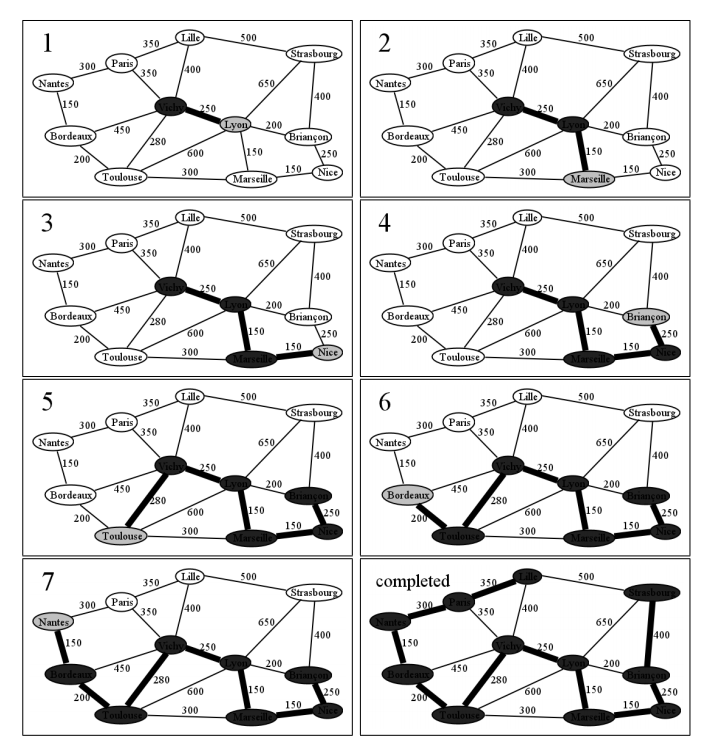
Let’s follow the algorithm’s progress in the WWII example. We can start with any node, so we’ll pick Vichy just at random. Frame 1 of Figure \(\PageIndex{12}\) shows what happens when the algorithm begins with Vichy: we simply examine all its neighbors, and connect the one that’s closest to it. Nothing could be simpler. In this case, Lyon is a mere 250 km away, which is closer than anything else is to Vichy, so we connect it and add the Vichy–Lyon edge to our edge set. The figure shows a heavy black line between Vichy and Lyon to show that it will officially be a supply line.
And so it goes. In successive frames, we add Marseille, Nice, and Briançon to the set of connected nodes, since we can do no better than 150 km, 150 km, and 250 km, respectively. Note that in frame 5 we do not darken the edge between Lyon and Briançon, even though 200 km is the shortest connected edge, because those nodes have already been previously connected. Note also that the algorithm can jump around from side to side — we aren’t looking for the shortest edge from the most recently added node, but rather the shortest edge from any connected node.
The final result is shown in the last frame. This is the best way to connect all the cities to each other, if “best" means “least total supply line distance." But if you look carefully, you’ll notice a fascinating thing. This network of edges does not contain the shortest path from Bordeaux to Strasbourg! I find that result dumbfounding. Wouldn’t you think that the shortest path between any two nodes would land right on this Prim network? Yet if you compare Figure \(\PageIndex{12}\) with Figure \(\PageIndex{11}\) you’ll see that the quickest way to Strasborg is directly through Marseille, not Vichy.
So we end up with the remarkable fact that the shortest route between two points has nothing whatsoever to do with the shortest total distance between all points. Who knew?
- The phrase “zero or more” is common in discrete math. In this case, it indicates that the empty graph, which contains no vertices at all, is still a legitimate graph.
- We’ll also say that a cycle can’t repeat any edges or vertices along the way, so that it can’t go back and forth repeatedly and pointlessly between two adjacent nodes. Some mathematicians call this a simple cycle to distinguish it from the more general cycle, but we’ll just say that no cycles can repeat like this.