5.2: Trees

A tree is really nothing but a simplification of a graph. There are two kinds of trees in the world: free trees, and rooted trees. ¹

Free trees

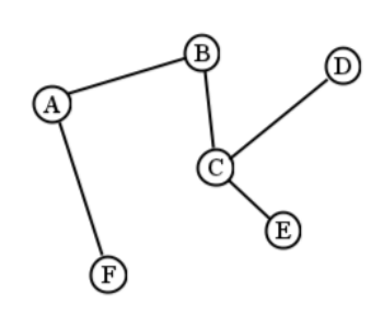
A free tree is just a connected graph with no cycles. Every node is reachable from the others, and there’s only one way to get anywhere. Take a look at Figure  \(\PageIndex{1}\) . It looks just like a graph (and it is) but unlike the WWII France graph, it’s more skeletal. This is because in some sense, a free tree doesn’t contain anything “extra."

Figure \(\PageIndex{1}\): A free tree.

If you have a free tree, the following interesting facts are true:

1. There’s exactly one path between any two nodes. (Check it!)

2. If you remove any edge, the graph becomes disconnected. (Try it!)

3. If you add any new edge, you end up adding a cycle. (Try it!)

4. [onelessedge] If there are \(n\) nodes, there are \(n-1\) edges. (Think about it!)

So basically, if your goal is connecting all the nodes, and you have a free tree, you’re all set. Adding anything is redundant, and taking away anything breaks it.

If this reminds you of Prim’s algorithm, it should. Prim’s algorithm produced exactly this: a free tree connecting all the nodes — and specifically the free tree with shortest possible total length. Go back and look at the final frame of Figure 5.1.12 and convince yourself that the darkened edges form a free tree.

For this reason, the algorithm is often called Prim’s minimal spanning tree algorithm. A “spanning tree" just means “a free tree that spans (connects) all the graph’s nodes."

Keep in mind that there are many free trees one can make with the same set of vertices. For instance, if you remove the edge from A to F, and add one from anything else to F, you have a different free tree.

Rooted trees

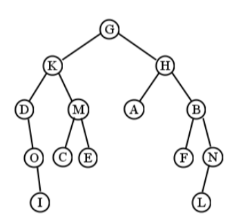
Now a rooted tree is the same thing as a free tree, except that we elevate one node to become the root. It turns out this makes all the difference. Suppose we chose A as the root of Figure  \(\PageIndex{1}\) . Then we would have the rooted tree in the left half of Figure  \(\PageIndex{2}\) . The A vertex has been positioned at the top, and everything else is flowing under it. I think of it as reaching into the free tree, carefully grasping a node, and then lifting up your hand so the rest of the free tree dangles from there. Had we chosen (say) C as the root instead, we would have a different rooted tree, depicted in the right half of the figure. Both of these rooted trees have all the same edges as the free tree did: B is connected to both A and C, F is connected only to A, etc. The only difference is which node is designated the root.

Up to now we’ve said that the spatial positioning on graphs is irrelevant. But this changes a bit with rooted trees. Vertical positioning is our only way of showing which nodes are “above" others, and the word “above" does indeed have meaning here: it means closer to the root. The altitude of a node shows how many steps it is away from the root. In the right rooted tree, nodes B, D, and E are all one step away from the root (C), while node F is three steps away.

Figure \(\PageIndex{2}\): Two different rooted trees with the same vertices and edges.

The key aspect to rooted trees — which is both their greatest advantage and greatest limitation — is that every node has one and only one path to the root. This behavior is inherited from free trees: as we noted, every node has only one path to every other.

Trees have a myriad of applications. Think of the files and folders on your hard drive: at the top is the root of the filesystem (perhaps “/" on Linux/Mac or “C:\\" on Windows) and underneath that are named folders. Each folder can contain files as well as other named folders, and so on down the hierarchy. The result is that each file has one, and only one, distinct path to it from the top of the filesystem. The file can be stored, and later retrieved, in exactly one way.

An “org chart" is like this: the CEO is at the top, then underneath her are the VP’s, the Directors, the Managers, and finally the rank-and-file employees. So is a military organization: the Commander in Chief directs generals, who command colonels, who command majors, who command captains, who command lieutenants, who command sergeants, who command privates.

The human body is even a rooted tree of sorts: it contains skeletal, cardiovascular, digestive, and other systems, each of which is comprised of organs, then tissues, then cells, molecules, and atoms. In fact, anything that has this sort of part-whole containment hierarchy is just asking to be represented as a tree.

In computer programming, the applications are too numerous to name. Compilers scan code and build a “parse tree" of its underlying meaning. HTML is a way of structuring plain text into a tree-like hierarchy of displayable elements. AI chess programs build trees representing their possible future moves and their opponent’s probable responses, in order to “see many moves ahead" and evaluate their best options. Object-oriented designs involve “inheritance hierarchies" of classes, each one specialized from a specific other. Etc. Other than a simple sequence (like an array), trees are probably the most common data structure in all of computer science.

Rooted tree terminology

Rooted trees carry with them a number of terms. I’ll use the tree on the left side of Figure  \(\PageIndex{2}\) as an illustration of each:

root.

The node at the top of the tree, which is A in our example. Note that unlike trees in the real world, computer science trees have their root at the top and grow down. Every tree has a root except the empty tree, which is the “tree" that has no nodes at all in it. (It’s kind of weird thinking of “nothing" as a tree, but it’s kind of like the empty set \(\varnothing\), which is still a set.)

parent.

Every node except the root has one parent: the node immediately above it. D’s parent is C, C’s parent is B, F’s parent is A, and A has no parent.

child.

Some nodes have children, which are nodes connected directly below it. A’s children are F and B, C’s are D and E, B’s only child is C, and E has no children.

sibling.

A node with the same parent. E’s sibling is D, B’s is F, and none of the other nodes have siblings.

ancestor.

Your parent, grandparent, great-grandparent, etc., all the way back to the root. B’s only ancestor is A, while E’s ancestors are C, B, and A. Note that F is not C’s ancestor, even though it’s above it on the diagram: there’s no connection from C to F, except back through the root (which doesn’t count).

descendent.

Your children, grandchildren, great-grandchildren, etc., all the way the leaves. B’s descendents are C, D and E, while A’s are F, B, C, D, and E.

leaf.

A node with no children. F, D, and E are leaves. Note that in a (very) small tree, the root could itself be a leaf.

internal node.

Any node that’s not a leaf. A, B, and C are the internal nodes in our example.

depth (of a node).

A node’s depth is the distance (in number of nodes) from it to the root. The root itself has depth zero. In our example, B is of depth 1, E is of depth 3, and A is of depth 0.

height (of a tree).

A rooted tree’s height is the maximum depth of any of its nodes; i.e., the maximum distance from the root to any node. Our example has a height of 3, since the “deepest" nodes are D and E, each with a depth of 3. A tree with just one node is considered to have a height of 0. Bizarrely, but to be consistent, we’ll say that the empty tree has height -1! Strange, but what else could it be? To say it has height 0 seems inconsistent with a one-node tree also having height 0. At any rate, this won’t come up much.

level.

All the nodes with the same depth are considered on the same “level." B and F are on level 1, and D and E are on level 3. Nodes on the same level are not necessarily siblings. If F had a child named G in the example diagram, then G and C would be on the same level (2), but would not be siblings because they have different parents. (We might call them “cousins" to continue the family analogy.)

subtree.

Finally, much of what gives trees their expressive power is their recursive nature. This means that a tree is made up of other (smaller) trees. Consider our example. It is a tree with a root of A. But the two children of A are each trees in their own right! F itself is a tree with only one node. B and its descendents make another tree with four nodes. We consider these two trees to be subtrees of the original tree. The notion of “root" shifts somewhat as we consider subtrees — A is the root of the original tree, but B is the root of the second subtree. When we consider B’s children, we see that there is yet another subtree, which is rooted at C. And so on. It’s easy to see that any subtree fulfills all the properties of trees, and so everything we’ve said above applies also to it.

Binary trees (BT’s)

The nodes in a rooted tree can have any number of children. There’s a special type of rooted tree, though, called a binary tree which we restrict by simply saying that each node can have at most two children. Furthermore, we’ll label each of these two children as the “left child" and “right child." (Note that a particular node might well have only a left child, or only a right child, but it’s still important to know which direction that child is.)

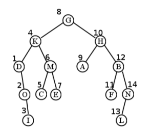
The left half of Figure \(\PageIndex{2}\) is a binary tree, but the right half is not (C has three children). A larger binary tree (of height 4) is shown in Figure  \(\PageIndex{3}\) .

Traversing binary trees

There were two ways of traversing a graph: breadth-first, and depth-first. Curiously, there are three ways of traversing a tree: pre-order, post-order, and in-order. All three begin at the root, and all three consider each of the root’s children as subtrees. The difference is in the order of visitation.

Figure \(\PageIndex{3}\): A binary tree.

To traverse a tree pre-order, we:

1. Visit the root.

2. Treat the left child and all its descendents as a subtree, and traverse it in its entirety.

3. Do the same with the right child.

It’s tricky because you have to remember that each time you “treat a child as a subtree" you do the whole traversal process on that subtree. This involves remembering where you were once you finish.

Follow this example carefully. For the tree in Figure  \(\PageIndex{3}\) , we begin by visiting G. Then, we traverse the whole “K subtree." This involves visiting K itself, and then traversing its whole left subtree (anchored at D). After we visit the D node, we discover that it actually has no left subtree, so we go ahead and traverse its right subtree. This visits O followed by I (since O has no left subtree either) which finally returns back up the ladder.

It’s at this point where it’s easy to get lost. We finish visiting I, and then we have to ask “okay, where the heck were we? How did we get here?" The answer is that we had just been at the K node, where we had traversed its left (D) subtree. So now what is it time to do? Traverse the right subtree, of course, which is M. This involves visiting M, C, and E (in that order) before returning to the very top, G.

Now we’re in the same sort of situation where we could have gotten lost before: we’ve spent a lot of time in the tangled mess of G’s left subtree, and we just have to remember that it’s now time to do G’s right subtree. Follow this same procedure, and the entire order of visitation ends up being: G, K, D, O, I, M, C, E, H, A, B, F, N, L. (See Figure  \(\PageIndex{4}\) for a visual.)

Figure \(\PageIndex{4}\): The order of node visitation in pre-order traversal.

To traverse a tree post-order, we:

1. Treat the left child and all its descendents as a subtree, and traverse it in its entirety.

2. Do the same with the right child.

3. Visit the root.

It’s the same as pre-order, except that we visit the root after the children instead of before. Still, despite its similarity, this has always been the trickiest one for me. Everything seems postponed, and you have to remember what order to do it in later.

For our sample tree, the first node visited turns out to be I. This is because we have to postpone visiting G until we finish its left (and right) subtree; then we postpone K until we finish its left (and right) subtree; postpone D until we’re done with O’s subtree, and postpone O until we do I. Then finally, the thing begins to unwind...all the way back up to K. But we can’t actually visit K itself yet, because we have to do its right subtree. This results in C, E, and M, in that order. Then we can do K, but we still can’t do G because we have its whole right subtree’s world to contend with. The entire order ends up being: I, O, D, C, E, M, K, A, F, L, N, B, H, and finally G. (See Figure  \(\PageIndex{5}\) for a visual.)

Note that this is not remotely the reverse of the pre-order visitation, as you might expect. G is last instead of first, but the rest is all jumbled up.

Figure \(\PageIndex{5}\): The order of node visitation in post-order traversal.

Finally, to traverse a tree in-order, we:

1. Treat the left child and all its descendents as a subtree, and traverse it in its entirety.

2. Visit the root.

3. Traverse the right subtree in its entirety.

So instead of visiting the root first (pre-order) or last (post-order) we treat it in between our left and right children. This might seem to be a strange thing to do, but there’s a method to the madness which will become clear in the next section.

For the sample tree, the first visited node is D. This is because it’s the first node encountered that doesn’t have a left subtree, which means step 1 doesn’t need to do anything. This is followed by O and I, for the same reason. We then visit K before its right subtree, which in turn visits C, M, and E, in that order. The final order is: D, O, I, K, C, M, E, G, A, H, F, B, L, N. (See Figure  \(\PageIndex{6}\) .)

If your nodes are spaced out evenly, you can read the in-order traversal off the diagram by moving your eyes left to right. Be careful about this, though, because ultimately the spatial position doesn’t matter, but rather the relationships between nodes. For instance, if I had drawn node I further to the right, in order to make the lines between D–O–I less steep, that I node might have been pushed physically to the right of K. But that wouldn’t change the order and have K visited earlier.

Figure \(\PageIndex{6}\): The order of node visitation in in-order traversal.

Finally, it’s worth mentioning that all of these traversal methods make elegant use of recursion. Recursion is a way of taking a large problem and breaking it up into similar, but smaller, subproblems. Then, each of those subproblems can be attacked in the same way as you attacked the larger problem: by breaking them up into subproblems. All you need is a rule for eventually stopping the “breaking up" process by actually doing something.

Every time one of these traversal processes treats a left or right child as a subtree, they are “recursing" by re-initiating the whole traversal process on a smaller tree. Pre-order traversal, for instance, after visiting the root, says, “okay, let’s pretend we started this whole traversal thing with the smaller tree rooted at my left child. Once that’s finished, wake me up so I can similarly start it with my right child." Recursion is a very common and useful way to solve certain complex problems, and trees are rife with opportunities.

Sizes of binary trees

Binary trees can be any ragged old shape, like our Figure  \(\PageIndex{3}\) example. Sometimes, though, we want to talk about binary trees with a more regular shape, that satisfy certain conditions. In particular, we’ll talk about three special kinds:

full binary tree.

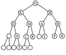
A full binary tree is one in which every node (except the leaves) has two children. Put another way, every node has either two children or none: no stringiness allowed. Figure  \(\PageIndex{3}\) is not full, but it would be if we added the three blank nodes in Figure  \(\PageIndex{7}\) .

Figure \(\PageIndex{7}\): A full binary tree.

By the way, it isn’t always possible to have a full binary tree with a particular number of nodes. For instance, a binary tree with two nodes, can’t be full, since it inevitably will have a root with only one child.

complete binary tree.

A complete binary tree is one in which every level has all possible nodes present, except perhaps for the deepest level, which is filled all the way from the left. Figure  \(\PageIndex{7}\) is not full, but it would be if we fixed it up as in Figure  \(\PageIndex{8}\) .

Figure \(\PageIndex{8}\): A complete binary tree.

Unlike full binary trees, it is always possible to have a complete binary tree no matter how many nodes it contains. You just keep filling in from left to right, level after level.

perfect binary tree.

Our last special type has a rather audacious title, but a “perfect" tree is simply one that is exactly balanced: every level is completely filled. Figure  \(\PageIndex{8}\) is not perfect, but it would be if we either added nodes to fill out level 4, or deleted the unfinished part of level 3 (as in Figure  \(\PageIndex{9}\) .)

Figure \(\PageIndex{9}\): A “perfect" binary tree.

Perfect binary trees obviously have the strictest size restrictions. It’s only possible, in fact, to have perfect binary trees with \(2^{h+1}-1\) nodes, if \(h\) is the height of the tree. So there are perfect binary trees with 1, 3, 7, 15, 31, ... nodes, but none in between. In each such tree, \(2^h\) of the nodes (almost exactly half) are leaves.

Now as we’ll see, binary trees can possess some pretty amazing powers if the nodes within them are organized in certain ways. Specifically, a binary search tree and a heap are two special kinds of binary trees that conform to specific constraints. In both cases, what makes them so powerful is the rate at which a tree grows as nodes are added to it.

Suppose we have a perfect binary tree. To make it concrete, let’s say it has height 3, which would give it 1+2+4+8=15 nodes, 8 of which are leaves. Now what happens if you increase the height of this tree to 4? If it’s still a “perfect" tree, you will have added 16 more nodes (all leaves). Thus you have doubled the number of leaves by simply adding one more level. This cascades the more levels you add. A tree of height 5 doubles the number of leaves again (to 32), and height 6 doubles it again (to 64).

If this doesn’t seem amazing to you, it’s probably because you don’t fully appreciate how quickly this kind of exponential growth can accumulate. Suppose you had a perfect binary tree of height 30 — certainly not an awe-inspiring figure. One could imagine it fitting on a piece of paper...height-wise, that is. But run the numbers and you’ll discover that such a tree would have over , more than one for every person in the United States. Increase the tree’s height to a mere 34 — just 4 additional levels — and suddenly you have over 8 billion leaves, easily greater than the population of planet Earth.

The power of exponential growth is only fully reached when the binary tree is perfect, since a tree with some “missing" internal nodes does not carry the maximum capacity that it’s capable of. It’s got some holes in it. Still, as long as the tree is fairly bushy (i.e., it’s not horribly lopsided in just a few areas) the enormous growth predicted for perfect trees is still approximately the case.

The reason this is called “exponential" growth is that the quantity we’re varying — the height — appears as an exponent in the number of leaves, which is \(2^h\). Every time we add just one level, we double the number of leaves.

So the number of leaves (call it \(l\)) is \(2^h\), if \(h\) is the height of the tree. Flipping this around, we say that \(h = \lg(l)\). The function “lg" is a logarithm, specifically a logarithm with base-2. This is what computer scientists often use, rather than a base of 10 (which is written “log") or a base of \(e\) (which is written “ln"). Since \(2^h\) grows very, very quickly, it follows that \(\lg(l)\) grows very, very slowly. After our tree reaches a few million nodes, we can add more and more nodes without growing the height of the tree significantly at all.

The takeaway message here is simply that an incredibly large number of nodes can be accommodated in a tree with a very modest height. This makes it possible to, among other things, search a huge amount of information astonishingly quickly...provided the tree’s contents are arranged properly.

Binary trees (BT’s)

The nodes in a rooted tree can have any number of children. There’s a special type of rooted tree, though, called a binary tree which we restrict by simply saying that each node can have at most two children. Furthermore, we’ll label each of these two children as the “left child" and “right child." (Note that a particular node might well have only a left child, or only a right child, but it’s still important to know which direction that child is.)

The left half of Figure  \(\PageIndex{9}\) is a binary tree, but the right half is not (C has three children). A larger binary tree (of height 4) is shown in Figure  \(\PageIndex{10}\) .

Traversing binary trees

There were two ways of traversing a graph: breadth-first, and depth-first. Curiously, there are three ways of traversing a tree: pre-order, post-order, and in-order. All three begin at the root, and all three consider each of the root’s children as subtrees. The difference is in the order of visitation.

Figure \(\PageIndex{10}\): A binary tree.

To traverse a tree pre-order, we:

1. Visit the root.

2. Treat the left child and all its descendents as a subtree, and traverse it in its entirety.

3. Do the same with the right child.

It’s tricky because you have to remember that each time you “treat a child as a subtree" you do the whole traversal process on that subtree. This involves remembering where you were once you finish.

Follow this example carefully. For the tree in Figure  \(\PageIndex{10}\) , we begin by visiting G. Then, we traverse the whole “K subtree." This involves visiting K itself, and then traversing its whole left subtree (anchored at D). After we visit the D node, we discover that it actually has no left subtree, so we go ahead and traverse its right subtree. This visits O followed by I (since O has no left subtree either) which finally returns back up the ladder.

It’s at this point where it’s easy to get lost. We finish visiting I, and then we have to ask “okay, where the heck were we? How did we get here?" The answer is that we had just been at the K node, where we had traversed its left (D) subtree. So now what is it time to do? Traverse the right subtree, of course, which is M. This involves visiting M, C, and E (in that order) before returning to the very top, G.

Now we’re in the same sort of situation where we could have gotten lost before: we’ve spent a lot of time in the tangled mess of G’s left subtree, and we just have to remember that it’s now time to do G’s right subtree. Follow this same procedure, and the entire order of visitation ends up being: G, K, D, O, I, M, C, E, H, A, B, F, N, L. (See Figure  \(\PageIndex{11}\) for a visual.)

Figure \(\PageIndex{11}\): The order of node visitation in pre-order traversal.

To traverse a tree post-order, we:

1. Treat the left child and all its descendents as a subtree, and traverse it in its entirety.

2. Do the same with the right child.

3. Visit the root.

It’s the same as pre-order, except that we visit the root after the children instead of before. Still, despite its similarity, this has always been the trickiest one for me. Everything seems postponed, and you have to remember what order to do it in later.

For our sample tree, the first node visited turns out to be I. This is because we have to postpone visiting G until we finish its left (and right) subtree; then we postpone K until we finish its left (and right) subtree; postpone D until we’re done with O’s subtree, and postpone O until we do I. Then finally, the thing begins to unwind...all the way back up to K. But we can’t actually visit K itself yet, because we have to do its right subtree. This results in C, E, and M, in that order. Then we can do K, but we still can’t do G because we have its whole right subtree’s world to contend with. The entire order ends up being: I, O, D, C, E, M, K, A, F, L, N, B, H, and finally G. (See Figure  \(\PageIndex{11}\) for a visual.)

Note that this is not remotely the reverse of the pre-order visitation, as you might expect. G is last instead of first, but the rest is all jumbled up.

Figure \(\PageIndex{12}\): The order of node visitation in post-order traversal.

Finally, to traverse a tree in-order, we:

1. Treat the left child and all its descendents as a subtree, and traverse it in its entirety.

2. Visit the root.

3. Traverse the right subtree in its entirety.

So instead of visiting the root first (pre-order) or last (post-order) we treat it in between our left and right children. This might seem to be a strange thing to do, but there’s a method to the madness which will become clear in the next section.

For the sample tree, the first visited node is D. This is because it’s the first node encountered that doesn’t have a left subtree, which means step 1 doesn’t need to do anything. This is followed by O and I, for the same reason. We then visit K before its right subtree, which in turn visits C, M, and E, in that order. The final order is: D, O, I, K, C, M, E, G, A, H, F, B, L, N. (See Figure  \(\PageIndex{13}\) .)

If your nodes are spaced out evenly, you can read the in-order traversal off the diagram by moving your eyes left to right. Be careful about this, though, because ultimately the spatial position doesn’t matter, but rather the relationships between nodes. For instance, if I had drawn node I further to the right, in order to make the lines between D–O–I less steep, that I node might have been pushed physically to the right of K. But that wouldn’t change the order and have K visited earlier.

Figure \(\PageIndex{13}\): The order of node visitation in in-order traversal.

Finally, it’s worth mentioning that all of these traversal methods make elegant use of recursion. Recursion is a way of taking a large problem and breaking it up into similar, but smaller, subproblems. Then, each of those subproblems can be attacked in the same way as you attacked the larger problem: by breaking them up into subproblems. All you need is a rule for eventually stopping the “breaking up" process by actually doing something.

Every time one of these traversal processes treats a left or right child as a subtree, they are “recursing" by re-initiating the whole traversal process on a smaller tree. Pre-order traversal, for instance, after visiting the root, says, “okay, let’s pretend we started this whole traversal thing with the smaller tree rooted at my left child. Once that’s finished, wake me up so I can similarly start it with my right child." Recursion is a very common and useful way to solve certain complex problems, and trees are rife with opportunities.

Sizes of binary trees

Binary trees can be any ragged old shape, like our Figure  \(\PageIndex{10}\) example. Sometimes, though, we want to talk about binary trees with a more regular shape, that satisfy certain conditions. In particular, we’ll talk about three special kinds:

full binary tree.

A full binary tree is one in which every node (except the leaves) has two children. Put another way, every node has either two children or none: no stringiness allowed. Figure  \(\PageIndex{10}\) is not full, but it would be if we added the three blank nodes in Figure \(\PageIndex{14}\) .

Figure \(\PageIndex{14}\): A full binary tree.

By the way, it isn’t always possible to have a full binary tree with a particular number of nodes. For instance, a binary tree with two nodes, can’t be full, since it inevitably will have a root with only one child.

complete binary tree.

A complete binary tree is one in which every level has all possible nodes present, except perhaps for the deepest level, which is filled all the way from the left. Figure  \(\PageIndex{14}\) is not full, but it would be if we fixed it up as in Figure \(\PageIndex{15}\).

Figure \(\PageIndex{15}\): A complete binary tree.

Unlike full binary trees, it is always possible to have a complete binary tree no matter how many nodes it contains. You just keep filling in from left to right, level after level.

perfect binary tree.

Our last special type has a rather audacious title, but a “perfect" tree is simply one that is exactly balanced: every level is completely filled. Figure  \(\PageIndex{15}\) is not perfect, but it would be if we either added nodes to fill out level 4, or deleted the unfinished part of level 3 (as in Figure  \(\PageIndex{16}\) .)

Figure \(\PageIndex{16}\): A “perfect" binary tree.

Perfect binary trees obviously have the strictest size restrictions. It’s only possible, in fact, to have perfect binary trees with \(2^{h+1}-1\) nodes, if \(h\) is the height of the tree. So there are perfect binary trees with 1, 3, 7, 15, 31, ... nodes, but none in between. In each such tree, \(2^h\) of the nodes (almost exactly half) are leaves.

Now as we’ll see, binary trees can possess some pretty amazing powers if the nodes within them are organized in certain ways. Specifically, a binary search tree and a heap are two special kinds of binary trees that conform to specific constraints. In both cases, what makes them so powerful is the rate at which a tree grows as nodes are added to it.

Suppose we have a perfect binary tree. To make it concrete, let’s say it has height 3, which would give it 1+2+4+8=15 nodes, 8 of which are leaves. Now what happens if you increase the height of this tree to 4? If it’s still a “perfect" tree, you will have added 16 more nodes (all leaves). Thus you have doubled the number of leaves by simply adding one more level. This cascades the more levels you add. A tree of height 5 doubles the number of leaves again (to 32), and height 6 doubles it again (to 64).

If this doesn’t seem amazing to you, it’s probably because you don’t fully appreciate how quickly this kind of exponential growth can accumulate. Suppose you had a perfect binary tree of height 30 — certainly not an awe-inspiring figure. One could imagine it fitting on a piece of paper...height-wise, that is. But run the numbers and you’ll discover that such a tree would have over , more than one for every person in the United States. Increase the tree’s height to a mere 34 — just 4 additional levels — and suddenly you have over 8 billion leaves, easily greater than the population of planet Earth.

The power of exponential growth is only fully reached when the binary tree is perfect, since a tree with some “missing" internal nodes does not carry the maximum capacity that it’s capable of. It’s got some holes in it. Still, as long as the tree is fairly bushy (i.e., it’s not horribly lopsided in just a few areas) the enormous growth predicted for perfect trees is still approximately the case.

The reason this is called “exponential" growth is that the quantity we’re varying — the height — appears as an exponent in the number of leaves, which is \(2^h\). Every time we add just one level, we double the number of leaves.

So the number of leaves (call it \(l\)) is \(2^h\), if \(h\) is the height of the tree. Flipping this around, we say that \(h = \lg(l)\). The function “lg" is a logarithm, specifically a logarithm with base-2. This is what computer scientists often use, rather than a base of 10 (which is written “log") or a base of \(e\) (which is written “ln"). Since \(2^h\) grows very, very quickly, it follows that \(\lg(l)\) grows very, very slowly. After our tree reaches a few million nodes, we can add more and more nodes without growing the height of the tree significantly at all.

The takeaway message here is simply that an incredibly large number of nodes can be accommodated in a tree with a very modest height. This makes it possible to, among other things, search a huge amount of information astonishingly quickly...provided the tree’s contents are arranged properly.

Binary search trees (BST’s)

Okay, then let’s talk about how to arrange those contents. A binary search tree (BST) is any binary tree that satisfies one additional property: every node is “greater than" all of the nodes in its left subtree, and “less than (or equal to)" all of the nodes in its right subtree. We’ll call this the BST property. The phrases “greater than" and “less than" are in quotes here because their meaning is somewhat flexible, depending on what we’re storing in the tree. If we’re storing numbers, we’ll use numerical order. If we’re storing names, we’ll use alphabetical order. Whatever it is we’re storing, we simply need a way to compare two nodes to determine which one “goes before" the other.

An example of a BST containing people is given in Figure  \(\PageIndex{17}\) . Imagine that each of these nodes contains a good deal of information about a particular person — an employee record, medical history, account information, what have you. The nodes themselves are indexed by the person’s name, and the nodes are organized according to the BST rule. Mitch comes after Ben/Jessica/Jim and before Randi/Owen/Molly/Xander in alphabetical order, and this ordering relationship between parents and children repeats itself all the way down the tree. (Check it!)

Be careful to observe that the ordering rule applies between a node and the entire contents of its subtrees, not merely to its immediate children. This is a rookie mistake that you want to avoid. Your first inclincation, when glancing at Figure \(\PageIndex{18}\) , below, is to judge it a BST. It is not a binary search tree, however! Jessica is to the left of Mitch, as she should be, and Nancy is to the right of Jessica, as she should be. It seems to check out. But the problem is that Nancy is a descendent of Mitch’s left subtree, whereas she must properly be placed somewhere in his right subtree. And yes, this matters. So be sure to check your BST’s all the way up and down.

Figure \(\PageIndex{17}\): A binary search tree.

Figure \(\PageIndex{18}\): NOT a binary search tree, though it looks like one at first glance. (Notice Nancy and Mitch)

The power of BST’s

All right, so what’s all the buzz about BST’s, anyway? The key insight is to realize that if you’re looking for a node, all you have to do is start at the root and go the height of the tree down making one comparison at each level. Let’s say we’re searching Figure \(\PageIndex{17}\) for Molly. By looking at Mitch (the root), we know right away that Molly must be in the right subtree, not the left, because she comes after Mitch in alphabetical order. So we look at Randi. This time, we find that Molly comes before Randi, so she must be somewhere in Randi’s left branch. Owen sends us left again, at which point we find Molly.

With a tree this size, it doesn’t seem that amazing. But suppose its height were 10. This would mean about 2000 nodes in the tree — customers, users, friends, whatever. With a BST, you’d only have to examine ten of those 2000 nodes to find whatever you’re looking for, whereas if the nodes were just in an ordinary list, you’d have to compare against 1000 or so of them before you stumbled on the one you were looking for. And as the size of the tree grows, this discrepancy grows (much) larger. If you wanted to find a single person’s records in New York City, would you rather search 7 million names, or 24 names?? Because that’s the difference you’re looking at.

It seems almost too good to be true. How is such a speedup possible? The trick is to realize that with every node you look at, you effectively eliminate half of the remaining tree from consideration. For instance, if we’re looking for Molly, we can disregard Mitch’s entire left half without even looking at it, then the same for Randi’s entire right half. If you discard half of something, then half of the remaining half, then half again, it doesn’t take you long before you’ve eliminated almost every false lead.

There’s a formal way to describe this speedup, called “Big-O notation." The subtleties are a bit complex, but the basic idea is this. When we say that an algorithm is “O(n)" (pronounced “oh–of–n"), it means that the time it takes to execute the algorithm is proportional to the number of nodes. This doesn’t imply any specific number of milliseconds or anything — that is highly dependent on the type of computer hardware, you have, the programming language, and a myriad of other things. But what we can say about an O(n) algorithm is that if you double the number of nodes, you’re going to approximately double the running time. If you quadruple the number of nodes, you’re going to quadruple the running time. This is what you’d expect.

Searching for “Molly" in a simple unsorted list of names is an O(n) prospect. If there’s a thousand nodes in the list, on average you’ll find Molly after scanning through 500 of them. (You might get lucky and find Molly at the beginning, but then of course you might get really unlucky and not find her until the end. This averages out to about half the size of the list in the normal case.) If there’s a million nodes, however, it’ll take you 500,000 traversals on average before finding Molly. Ten times as many nodes means ten times as long to find Molly, and a thousand times as many means a thousand times as long. Bummer.

Looking up Molly in a BST, however, is an O(lg n) process. Recall that “lg" means the logarithm (base-2). This means that doubling the number of nodes gives you a miniscule increase in the running time. Suppose there were a thousand nodes in your tree, as above. You wouldn’t have to look through 500 to find Molly: you’d only have to look through ten (because \(\lg(1000) \approx 10\)). Now increase it to a million nodes. You wouldn’t have to look through 500,000 to find Molly: you’d only have to look through twenty. Suppose you had 6 billion nodes in your tree (approximately the population of the earth). You wouldn’t have to look through 3 billion nodes: you’d only have to look through thirty-three. Absolutely mind-boggling.

Adding nodes to a BST

Finding things in a BST is lightning fast. Turns out, so is adding things to it. Suppose we acquire a new customer named Jennifer, and we need to add her to our BST so we can retrieve her account information in the future. All we do is follow the same process we would if we were looking for Jennifer, but as soon as we find the spot where she would be, we add her there. In this case, Jennifer comes before Mitch (go left), and before Jessica (go left again), and after Ben (go right). Ben has no right child, so we put Jessica in the tree right at that point. (See Figure  \(\PageIndex{19}\) .)

This adding process is also an O(lg n) algorithm, since we only need look at a small number of nodes equal to the height of the tree.

Figure \(\PageIndex{19}\): The BST after adding Jennifer.

Note that a new entry always becomes a leaf when added. In fact, this allows us to look at the tree and reconstruct some of what came before. For instance, we know that Mitch must have been the first node originally inserted, and that Randi was inserted before Owen, Xander, or Molly. As an exercise, add your own name to this tree (and a few of your friends’ names) to make sure you get the hang of it. When you’re done the tree must of course obey the BST property.

Removing nodes from a BST

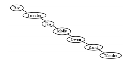
Removing nodes is a bit trickier than adding them. How do we delete an entry without messing up the structure of the tree? It’s easy to see how to delete Molly: since she’s just a leaf, just remove her and be done with it. But how to delete Jessica? Or for that matter, Mitch?

Your first inclination might be to eliminate a node and promote one of its children to go up in its place. For instance, if we delete Jessica, we could just elevate Ben up to where Jessica was, and then move Jennifer up under Ben as well. This doesn’t work, though. The result would look like Figure  \(\PageIndex{20}\) , with Jennifer in the wrong place. The next time we look for Jennifer in the tree, we’ll search to the right of Ben (as we should), completely missing her. Jennifer has effectively been lost.

One correct way (there are others) to do a node removal is to replace the node with the left-most descendent of its right subtree. (Or, equivalently, the right-most descendent of its left subtree). Figure  \(\PageIndex{21}\) shows the result after removing Jessica. We replaced her with Jim, not because it’s okay to blindly promote the right child, but because Jim had no left descendents. If he had, promoting him would have been just as wrong as promoting Ben. Instead, we would have promoted Jim’s left-most descendent.

Figure \(\PageIndex{20}\): An incorrect would-be-BST after removing Jessica incorrectly.

Figure \(\PageIndex{21}\): The BST after removing Jessica correctly.

As another example, let’s go whole-hog and remove the root node, Mitch. The result is as shown in Figure  \(\PageIndex{22}\) . It’s rags-to-riches for Molly: she got promoted from a leaf all the way to the top. Why Molly? Because she was the left-most descendent of Mitch’s right subtree.

To see why this works, just consider that Molly was immediately after Mitch in alphabetical order. The fact that he was a king and she a peasant was misleading. The two of them were actually very close: consecutive, in fact, with in-order traversal. So replacing Mitch with Molly avoids shuffling anybody out of alphabetical order, and preserves the all-important BST property.

Figure \(\PageIndex{22}\): The BST after removing Mitch.

Balancedness

Finally, recall that this amazingly fast lookup is critically dependent on the tree being “bushy." Otherwise, the approximation that \(h=\lg(l)\) breaks down. As a laughably extreme example, consider Figure \(\PageIndex{23}\) , which contains the same nodes we’ve been using. This is a legitimate binary search tree! (Check it!) Yet looking up a node in this monstrosity is obviously not going to be any faster than looking it up in a plain-old list. We’re back to O(n) performance.

Figure \(\PageIndex{23}\): An incredibly bad, but still technically legit, BST.

In practice, there are three ways of dealing with this. One approach is to simply not worry about it. After all, as long as we’re inserting and removing nodes randomly, with no discernable pattern, the chances of obtaining a tree as lopsided as Figure  \(\PageIndex{23}\) are astronomically small. It’s as likely as throwing a deck of cards up in the air and having it land all in a neat stack. The law of entropy tells us that we’re going to get a mix of short branches and long branches, and that in a large tree, the unbalancedness will be minimal.

A second approach is to periodically rebalance the tree. If our website goes offline for maintenance every once in a while anyway, we could rebuild our tree from the ground up by inserting the nodes into a fresh tree in a beneficial order. What order should we insert them in? Well, remember that whichever node is inserted first will be the root. This suggests that we’d want to insert the middle node first into our tree, so that Molly becomes the new root. This leaves half the nodes for her left subtree and half for her right. If you follow this process logically (and recursively) you’ll realize that we’d next want to insert the middle nodes of each half. This would equate to Jennifer and Randi (in either order). I think of it like the markings on a ruler: first you insert half an inch, then \(\frac{1}{4}\) and \(\frac{3}{4}\) inches, then \(\frac{1}{8}\), \(\frac{3}{8}\), \(\frac{5}{8}\), and \(\frac{7}{8}\) inches, etc. This restores to us a perfectly balanced tree at regular intervals, making any large imbalances even more improbably (and short-lived).

Thirdly, there are specialized data structures you may learn about in future courses, such as AVL trees and red-black trees, which are binary search trees that add extra rules to prevent imbalancing. Basically, the idea is that when a node is inserted (or removed), certain metrics are checked to make sure that the change didn’t cause too great an imbalance. If it did, the tree is adjusted so as to minimize the imbalance. This comes at a slight cost every time the tree is changed, but prevents any possibility of a lopsided tree that would cause slow lookups in the long run.

---

1. There appears to be no consensus as to which of these concepts is the most basic. Some authors refer to a free tree simply as a “tree” — as though this were the “normal” kind of tree — and use the term rooted tree for the other kind. Other authors do the opposite. To avoid confusion, I’ll try to always use the full term (although I admit I’m one who considers rooted trees to be the more important, default concept).