12.3: An Introduction to Vector Spaces

Motivation for the Study of Vector Spaces

When we encountered various types of matrices in Chapter 5, it became apparent that a particular kind of matrix, the diagonal matrix, was much easier to use in computations. For example, if \(A =\left( \begin{array}{cc} 2 & 1 \\ 2 & 3 \\ \end{array} \right)\text{,}\) then \(A^5\) can be found, but its computation is tedious. If \(D =\left( \begin{array}{cc} 1 & 0 \\ 0 & 4 \\ \end{array} \right)\) then

\begin{equation*} D^5 =\left( \begin{array}{cc} 1 & 0 \\ 0 & 4 \\ \end{array} \right)^5= \left( \begin{array}{cc} 1^5 & 0 \\ 0 & 4^5 \\ \end{array} \right)= \left( \begin{array}{cc} 1 & 0 \\ 0 & 1024 \\ \end{array} \right) \end{equation*}

Even when presented with a non-diagonal matrix, we will see that it is sometimes possible to do a bit of work to be able to work with a diagonal matrix. This process is called diagonalization.

In a variety of applications it is beneficial to be able to diagonalize a matrix. In this section we will investigate what this means and consider a few applications. In order to understand when the diagonalization process can be performed, it is necessary to develop several of the underlying concepts of linear algebra.

Vector Spaces

By now, you realize that mathematicians tend to generalize. Once we have found a “good thing,” something that is useful, we apply it to as many different concepts as possible. In doing so, we frequently find that the “different concepts” are not really different but only look different. Four sentences in four different languages might look dissimilar, but when they are translated into a common language, they might very well express the exact same idea.

Early in the development of mathematics, the concept of a vector led to a variety of applications in physics and engineering. We can certainly picture vectors, or “arrows,” in the \(x y-\textrm{ plane}\) and even in the three-dimensional space. Does it make sense to talk about vectors in four-dimensional space, in ten-dimensional space, or in any other mathematical situation? If so, what is the essence of a vector? Is it its shape or the rules it follows? The shape in two- or three-space is just a picture, or geometric interpretation, of a vector. The essence is the rules, or properties, we wish vectors to follow so we can manipulate them algebraically. What follows is a definition of what is called a vector space. It is a list of all the essential properties of vectors, and it is the basic definition of the branch of mathematics called linear algebra.

Definition \(\PageIndex{1}\): Vector Space

Let \(V\) be any nonempty set of objects. Define on \(V\) an operation, called addition, for any two elements \(\vec{x}, \vec{y} \in V\text{,}\) and denote this operation by \(\vec{x}+ \vec{y}\text{.}\) Let scalar multiplication be defined for a real number \(a \in \mathbb{R}\) and any element \(\vec{x}\in V\) and denote this operation by \(a \vec{x}\text{.}\) The set \(V\) together with operations of addition and scalar multiplication is called a vector space over \(\mathbb{R}\) if the following hold for all \(\vec{x}, \vec{y}, \vec{z}\in V\) , and \(a,b \in \mathbb{R}\text{:}\)

• \(\displaystyle \vec{x}+ \vec{y}= \vec{y}+ \vec{x}\)
• \(\displaystyle \left(\vec{x}+ \vec{y}\right)+ \vec{z}= \vec{x}+\left( \vec{y}+\vec{z}\right)\)
• There exists a vector \(\vec{0}\in V\text{,}\) such that \(\vec{x}+\vec{0} = \vec{x}\) for all \(x \in V\text{.}\)
• For each vector \(\vec{x}\in V\text{,}\) there exists a unique vector \(-\vec{x}\in V\text{,}\) such that \(-\vec{x} +\vec{x}= \vec{0}\text{.}\)

These are the main properties associated with the operation of addition. They can be summarized by saying that \([V; +]\) is an abelian group.

The next four properties are associated with the operation of scalar multiplication and how it relates to vector addition.

• \(\displaystyle a\left(\vec{x}+ \vec{y} \right) =a \vec{x}+a \vec{y}\)
• \(\displaystyle (a +b)\vec{x}= a \vec{x} + b \vec{x}\)
• \(\displaystyle a \left(b \vec{x}\right) = (a b)\vec{x}\)
• \(1\vec{x} = \vec{x}\text{.}\)

In a vector space it is common to call the elements of \(V\) vectors and those from \(\mathbb{R}\) scalars. Vector spaces over the real numbers are also called real vector spaces.

Example \(\PageIndex{1}\): A Vector Space of Matrices

Let \(V = M_{2\times 3}(\mathbb{R})\) and let the operations of addition and scalar multiplication be the usual operations of addition and scalar multiplication on matrices. Then \(V\) together with these operations is a real vector space. The reader is strongly encouraged to verify the definition for this example before proceeding further (see Exercise \(\PageIndex{3}\) of this section). Note we can call the elements of \(M_{2\times 3}(\mathbb{R})\) vectors even though they are not arrows.

Example \(\PageIndex{2}\): The Vector Space \(\mathbb{R}^{2}\)

Let \(\mathbb{R}^2 = \left\{\left(a_1, a_2 \right) \mid a_1,a_2 \in \mathbb{R}\right\}\text{.}\) If we define addition and scalar multiplication the natural way, that is, as we would on \(1\times 2\) matrices, then \(\mathbb{R}^2\) is a vector space over \(\mathbb{R}\text{.}\) See Exercise \(\PageIndex{4}\) of this section.

In this example, we have the “bonus” that we can illustrate the algebraic concept geometrically. In mathematics, a “geometric bonus” does not always occur and is not necessary for the development or application of the concept. However, geometric illustrations are quite useful in helping us understand concepts and should be utilized whenever available.

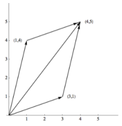Figure \(\PageIndex{1}\): Sum of two vectors in \(\mathbb{R}^{2}\)

Let's consider some illustrations of the vector space \(\mathbb{R}^2\text{.}\) Let \(\vec{x}= (1, 4)\) and \(\vec{y} = (3, 1)\text{.}\) We illustrate the vector \(\left(a_1, a_2\right)\) as a directed line segment, or “arrow,” from the point \((0, 0)\) to the point\(\left(a_1, a_2\right)\text{.}\) The vectors \(\vec{x}\) and \(\vec{y}\) are as shown in Figure \(\PageIndex{1}\) together with \(\vec{x}+ \vec{y} = (1, 4) + (3, 1) = (4, 5)\text{.}\) The vector \(2 \vec{x} = 2(1, 4) = (2, 8)\) is a vector in the same direction as \(\vec{x}\text{,}\) but with twice its length.

Note \(\PageIndex{1}\)

1. The common convention is to use that boldface letters toward the end of the alphabet for vectors, while letters early in the alphabet are scalars.
2. A common alternate notation for vectors is to place an arrow about a variable to indicate that it is a vector such as this: \(\overset{\rightharpoonup }{x}\text{.}\)
3. The vector \(\left(a_1,a_2,\ldots ,a_n\right)\in \mathbb{R}^n\) is referred to as an \(n\)-tuple.
4. For those familiar with vector calculus, we are expressing the vector \(x = a_1 \boldsymbol{\hat{\textbf{i}}}+ a_2 \boldsymbol{\hat{\textbf{j}}} + a_3 \boldsymbol{\hat{\textbf{k}}} \in \mathbb{R}^3\) as \(\left(a_1,a_2,a_3\right)\text{.}\) This allows us to discuss vectors in \(\mathbb{R}^n\) in much simpler notation.

In many situations a vector space \(V\) is given and we would like to describe the whole vector space by the smallest number of essential reference vectors. An example of this is the description of \(\mathbb{R}^2\text{,}\) the \(x y\)-plane, via the \(x\) and \(y\) axes. Again our concepts must be algebraic in nature so we are not restricted solely to geometric considerations.

Definition \(\PageIndex{2}\): Linear Combination

A vector \(\pmb{ y}\) in vector space \(V\) (over \(\mathbb{R}\)) is a linear combination of the vectors \(\vec{x}_1\text{,}\) \(\vec{x}_2, \ldots\text{,}\) \(\vec{x}_n\) if there exist scalars \(a_1,a_2,\ldots ,a_n\) in \(\mathbb{R}\) such that \(\vec{y} = a_1\vec{x}_1+ a_2\vec{x}_2+\ldots +a_n\vec{x}_n\)

Example \(\PageIndex{3}\): A Basic Example

The vector \((2, 3)\) in \(\mathbb{R}^2\) is a linear combination of the vectors \((1, 0)\) and \((0, 1)\) since \((2, 3) = 2(1, 0) + 3(0, 1)\text{.}\)

Example \(\PageIndex{4}\): A Little Less Obvious Example

Prove that the vector \((4,5)\) is a linear combination of the vectors (3, 1) and (1, 4).

By the definition we must show that there exist scalars \(a_1\) and \(a_2\) such that:

\begin{equation*} \begin{array}{ccc} \begin{split} (4,5) &= a_1(3, 1) + a_2 (1, 4)\\ & = \left(3a_1+ a_2 , a_1+4a_2\right) \end{split} &\Rightarrow & \begin{array}{c} 3a_1+ a_2 =4\\ a_1+ 4a_2 =5\\ \end{array}\\ \\ \end{array} \end{equation*}

This system has the solution \(a_1=1\text{,}\) \(a_2=1\text{.}\)

Hence, if we replace \(a_1\) and \(a_2\) both by 1, then the two vectors (3, 1) and (1, 4) produce, or generate, the vector (4,5). Of course, if we replace \(a_1\) and \(a_2\) by different scalars, we can generate more vectors from \(\mathbb{R}^2\text{.}\) If, for example, \(a _1 = 3\) and \(a_2 = -2\text{,}\) then

\begin{equation*} a_1(3, 1) + a_2 (1, 4) = 3 (3, 1) +(-2) (1,4) = (9, 3) +(-2,-8) = (7, -5) \end{equation*}

Will the vectors \((3, 1)\) and \((1,4)\) generate any vector we choose in \(\mathbb{R}^2\text{?}\) To see if this is so, we let \(\left(b_1,b_2\right)\) be an arbitrary vector in \(\mathbb{R}^2\) and see if we can always find scalars \(a_1\) and \(a_2\) such that \(a_1(3, 1) + a_2 (1, 4)= \left(b_1,b_2\right)\text{.}\) This is equivalent to solving the following system of equations:

\begin{equation*} \begin{array}{c} 3a_1+ a_2 =b_1\\ a_1+4a_2 =b_2\\ \end{array} \end{equation*}

which always has solutions for \(a_1\) and \(a_2\) , regardless of the values of the real numbers \(b_1\) and \(b_2\text{.}\) Why? We formalize this situation in a definition:

Definition \(\PageIndex{3}\): Generation of a Vector Space

Let \(\left\{\vec{x}_1,\vec{x}_2, \ldots ,\vec{x}_n\right\}\) be a set of vectors in a vector space \(V\) over \(\mathbb{R}\text{.}\) This set is said to generate, or span, \(V\) if, for any given vector \(\vec{y} \in V\text{,}\) we can always find scalars \(a_1\text{,}\) \(a_2, \ldots\text{,}\) \(a_n\) such that \(\vec{y} = a_1 \vec{x}_1+a_2 \vec{x}_2+\ldots +a_n \vec{x}_n\text{.}\) A set that generates a vector space is called a generating set.

We now give a geometric interpretation of the previous examples.

We know that the standard coordinate system, \(x\) axis and \(y\) axis, were introduced in basic algebra in order to describe all points in the \(xy\)-plane algebraically. It is also quite clear that to describe any point in the plane we need exactly two axes.

We can set up a new coordinate system in the following way. Draw the vector \((3, 1)\) and an axis from the origin through (3, 1) and label it the \(x'\) axis. Also draw the vector \((1,4)\) and an axis from the origin through \((1,4)\) to be labeled the \(y'\) axis. Draw the coordinate grid for the axis, that is, lines parallel, and let the unit lengths of this “new” plane be the lengths of the respective vectors, \((3, 1)\) and \((1, 4)\text{,}\) so that we obtain Figure \(\PageIndex{2}\).

From Example \(\PageIndex{4}\) and Figure \(\PageIndex{2}\), we see that any vector on the plane can be described using the standard \(xy\)-axes or our new \(x'y'\)-axes. Hence the position which had the name \((3,1)\) in reference to the standard axes has the name \((1,0)\) with respect to the \(x'y'\) axes, or, in the phraseology of linear algebra, the coordinates of the point \((1,4)\) with respect to the \(x'y'\) axes are \((1, 0)\text{.}\)

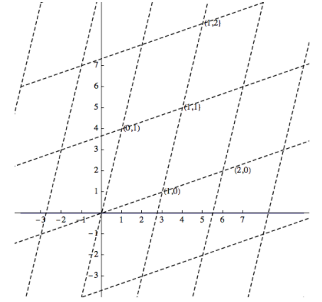Figure \(\PageIndex{2}\): Two sets of axes for the plane

Example \(\PageIndex{5}\): One Point, Two Position Descriptions

From Example \(\PageIndex{4}\) we found that if we choose \(a_1=1\) and \(a_2=1\text{,}\) then the two vectors \((3, 1)\) and \((1,4)\) generate the vector \((4,5)\text{.}\) Another geometric interpretation of this problem is that the coordinates of the position \((4,5)\) with respect to the \(x'y'\) axes of Figure \(\PageIndex{2}\) is \((1, 1)\text{.}\) In other words, a position in the plane has the name \((4,5)\) in reference to the \(xy\)-axes and the same position has the name \((1, 1)\) in reference to the \(x'y'\) axes.

From the above, it is clear that we can use different axes to describe points or vectors in the plane. No matter what choice we use, we want to be able to describe each position in a unique manner. This is not the case in Figure \(\PageIndex{3}\). Any point in the plane could be described via the \(x'y'\) axes, the \(x'z'\) axes or the \(y'z'\) axes. Therefore, in this case, a single point would have three different names, a very confusing situation.

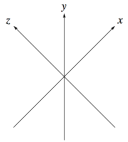Figure \(\PageIndex{3}\): Three axes on a plane

We formalize the our observations in the previous examples in two definitions and a theorem.

Definition \(\PageIndex{4}\): Linear Independence/Linear Dependence

A set of vectors \(\left\{\vec{x}_1,\vec{x}_2, \ldots ,\vec{x}_n\right\}\) from a real vector space \(V\) is linearly independent if the only solution to the equation \(a_1 \vec{x}_1+a_2 \vec{x}_2+\ldots +a_n \vec{x}_n= \vec{0}\) is \(a_1 = a_2 = \ldots = a_n = 0\text{.}\) Otherwise the set is called a linearly dependent set.

Definition \(\PageIndex{5}\): Basis

A set of vectors \(B=\left\{\vec{x}_1,\vec{x}_2, \ldots ,\vec{x}_n\right\}\) is a basis for a vector space \(V\) if:

1. \(B\) generates \(V\text{,}\) and
2. \(B\) is linearly independent.

Theorem \(\PageIndex{1}\): The Fundamental Property of a Basis

If \(\left\{\vec{x}_1,\vec{x}_2, \ldots ,\vec{x}_n\right\}\) is a basis for a vector space V over \(\mathbb{R}\text{,}\) then any vector \(y \in V\) can be uniquely expressed as a linear combination of the \(\vec{x}_i\textrm{'s}\text{.}\)

Proof

Assume that \(\left\{\vec{x}_1,\vec{x}_2, \ldots ,\vec{x}_n\right\}\) is a basis for \(V\) over \(\mathbb{R}\text{.}\) We must prove two facts:

1. each vector \(y \in V\) can be expressed as a linear combination of the \(\vec{x}_i\textrm{'s}\text{,}\) and
2. each such expression is unique.

Part 1 is trivial since a basis, by its definition, must generate all of \(V\text{.}\)

The proof of part 2 is a bit more difficult. We follow the standard approach for any uniqueness facts. Let \(y\) be any vector in \(V\) and assume that there are two different ways of expressing \(y\text{,}\) namely

\begin{equation*} y = a_1 \vec{x}_1+a_2 \vec{x}_2+\ldots +a_n \vec{x}_n \end{equation*}

and

\begin{equation*} y = b_1 \vec{x}_1+b_2 \vec{x}_2+\ldots +b_n \vec{x}_n \end{equation*}

where at least one \(a_i\) is different from the corresponding \(b_i\text{.}\) Then equating these two linear combinations we get

\begin{equation*} a_1 \vec{x}_1+a_2 \vec{x}_2+\ldots +a_n \vec{x}_n=b_1 \vec{x}_1+b_2 \vec{x}_2+\ldots +b_n \vec{x}_n \end{equation*}

so that

\begin{equation*} \left(a_1-b_1\right) \vec{x}_1+\left(a_2-b_2\right) \vec{x}_2+\ldots +\left(a_n-b_n\right) \vec{x}_n=\vec{0} \end{equation*}

Now a crucial observation: since the \(\vec{x}_i's\) form a linearly independent set, the only solution to the previous equation is that each of the coefficients must equal zero, so \(a_i-b_i=0\) for \(i = 1, 2, \ldots ,n\text{.}\) Hence \(a_i=b_i\text{,}\) for all \(i\text{.}\) This contradicts our assumption that at least one \(a_i\) is different from the corresponding \(b_i\text{,}\) so each vector \(\vec{y} \in V\) can be expressed in one and only one way.

This theorem, together with the previous examples, gives us a clear insight into the significance of linear independence, namely uniqueness in representing any vector.

Example \(\PageIndex{6}\): Another Basis for \(\mathbb{R}^{2}\)

Prove that \(\{(1, 1), (-1, 1)\}\) is a basis for \(\mathbb{R}^2\) over \(\mathbb{R}\) and explain what this means geometrically.

First we show that the vectors \((1, 1)\) and \((-1, 1)\) generate all of \(\mathbb{R}^2\text{.}\) We can do this by imitating Example \(\PageIndex{4}\) and leave it to the reader (see Exercise \(\PageIndex{10}\) of this section). Secondly, we must prove that the set is linearly independent.

Let \(a_1\) and \(a_2\) be scalars such that \(a_1 (1, 1) + a_2 (-1, 1) = (0, 0)\text{.}\) We must prove that the only solution to the equation is that \(a_1\) and \(a_2\) must both equal zero. The above equation becomes \(\left(a_1- a_2 , a_1 + a_2 \right) = (0, 0)\) which gives us the system

\begin{equation*} \begin{array}{c} a_1 - a_{2 }=0 \\ a_1 + a_2=0\\ \end{array} \end{equation*}

The augmented matrix of this system reduces in such way that the only solution is the trivial one of all zeros:

\begin{equation*} \left( \begin{array}{cc|c} 1 & -1 & 0 \\ 1 & 1 & 0 \\ \end{array} \right)\longrightarrow \left( \begin{array}{cc|c} 1 & 0 & 0 \\ 0 & 1 & 0 \\ \end{array} \right)\textrm{ }\Rightarrow \textrm{ }a_1 = a_2 =0 \end{equation*}

Therefore, the set is linearly independent.

To explain the results geometrically, note through Exercise 12, part a, that the coordinates of each vector \(\vec{y} \in \mathbb{R}^2\) can be determined uniquely using the vectors (1,1) and (-1, 1). The concept of dimension is quite obvious for those vector spaces that have an immediate geometric interpretation. For example, the dimension of \(\mathbb{R}^2\) is two and that of \(\mathbb{R}^3\) is three. How can we define the concept of dimension algebraically so that the resulting definition correlates with that of \(\mathbb{R}^2\) and \(\mathbb{R}^3\text{?}\) First we need a theorem, which we will state without proof.

Theorem \(\PageIndex{2}\): Basis Size is Constant

If \(V\) is a vector space with a basis containing \(n\) elements, then all bases of \(V\) contain \(n\) elements.

Definition \(\PageIndex{6}\): Dimension of a Vector Space

Let \(V\) be a vector space over \(\mathbb{R}\) with basis \(\left\{\vec{x}_1,\vec{x}_2, \ldots ,\vec{x}_n\right\}\text{.}\) Then the dimension of \(V\) is \(n\text{.}\) We use the notation \(\dim V = n\) to indicate that \(V\) is \(n\)-dimensional.

Exercises

Exercise \(\PageIndex{1}\)

If \(a = 2\text{,}\) \(b = -3\text{,}\) \(A=\left( \begin{array}{ccc} 1 & 0 & -1 \\ 2 & 3 & 4 \\ \end{array} \right)\text{,}\) \(B=\left( \begin{array}{ccc} 2 & -2 & 3 \\ 4 & 5 & 8 \\ \end{array} \right)\text{,}\) and \(C=\left( \begin{array}{ccc} 1 & 0 & 0 \\ 3 & 2 & -2 \\ \end{array} \right)\) verify that all properties of the definition of a vector space are true for \(M_{2\times 3}(\mathbb{R})\) with these values.

Exercise \(\PageIndex{2}\)

Let \(a = 3\text{,}\) \(b = 4\text{,}\) \(\vec{x}\pmb = (-1, 3)\text{,}\) \(\vec{y} = (2, 3)\text{,}\)and \(\vec{z} = (1, 0)\text{.}\) Verify that all properties of the definition of a vector space are true for \(\mathbb{R}^2\) for these values.

Exercise \(\PageIndex{3}\)

1. Verify that \(M_{2\times 3}(\mathbb{R})\) is a vector space over \(\mathbb{R}\text{.}\) What is its dimension?
2. Is \(M_{m\times n}(\mathbb{R})\) a vector space over \(\mathbb{R}\text{?}\) If so, what is its dimension?

Answer

The dimension of \(M_{2\times 3}(\mathbb{R})\) is 6 and yes, \(M_{m\times n}(\mathbb{R})\) is also a vector space of dimension \(m \cdot n\text{.}\) One basis for \(M_{m\times n}(\mathbb{R})\) is \(\{A_{ij} \mid 1 \leq i \leq m, 1 \leq j \leq n\}\) where \(A_{ij}\) is the \(m\times n\) matrix with entries all equal to zero except for in row \(i\text{,}\) column \(j\) where the entry is 1.

Exercise \(\PageIndex{4}\)

1. Verify that \(\mathbb{R}^2\) is a vector space over \(\mathbb{R}\text{.}\)
2. Is \(\mathbb{R}^n\) a vector space over \(\mathbb{R}\) for every positive integer \(n\text{?}\)

Exercise \(\PageIndex{5}\)

Let \(P^3= \left\{a_0 + a_1x + a_2x^2 + a_3x^3 \mid a_0,a_1,a_2,a_3\in \mathbb{R}\right\}\text{;}\) that is, \(P^3\) is the set of all polynomials in \(x\) having real coefficients with degree less than or equal to three. Verify that \(P^3\) is a vector space over \(\mathbb{R}\text{.}\) What is its dimension?

Exercise \(\PageIndex{6}\)

For each of the following, express the vector \(\pmb{y}\) as a linear combination of the vectors \(x_1\) and \(x_2\text{.}\)

1. \(\vec{y} = (5, 6)\text{,}\) \(\vec{x}_1 =(1, 0)\text{,}\) and \(\vec{x}_2 = (0, 1)\)
2. \(\vec{y} = (2, 1)\text{,}\) \(\vec{x}_1 =(2, 1)\text{,}\) and \(\vec{x}_2 = (1, 1)\)
3. \(\vec{y} = (3,4)\text{,}\) \(\vec{x}_1 = (1, 1)\text{,}\) and \(\vec{x}_2 = (-1, 1)\)

Exercise \(\PageIndex{7}\)

Express the vector \(\left( \begin{array}{cc} 1 & 2 \\ -3 & 3 \\ \end{array} \right)\in M_{2\times 2}(\mathbb{R})\text{,}\) as a linear combination of \(\left( \begin{array}{cc} 1 & 1 \\ 1 & 1 \\ \end{array} \right)\text{,}\) \(\left( \begin{array}{cc} -1 & 5 \\ 2 & 1 \\ \end{array} \right)\text{,}\) \(\left( \begin{array}{cc} 0 & 1 \\ 1 & 1 \\ \end{array} \right)\) and \(\left( \begin{array}{cc} 0 & 0 \\ 0 & 1 \\ \end{array} \right)\)

Answer

If the matrices are named \(B\text{,}\) \(A_1\text{,}\) \(A_2\) , \(A_3\text{,}\) and \(A_4\) , then

\begin{equation*} B = \frac{8}{3}A_1 + \frac{5}{3}A_2+\frac{-5}{3}A_3+\frac{23}{3}A_4 \end{equation*}

Exercise \(\PageIndex{8}\)

Express the vector \(x^3-4x^2+3\in P^3\) as a linear combination of the vectors 1, \(x\text{,}\) \(x^2\) , and \(x^3\text{.}\)

Exercise \(\PageIndex{9}\)

1. Show that the set \(\left\{\vec{x}_1,\vec{x}_2\right\}\) generates \(\mathbb{R}^2\) for each of the parts in Exercise \(\PageIndex{6}\) of this section.
2. Show that \(\left\{\vec{x}_1,\vec{x}_2,\vec{x}_3\right\}\) generates \(\mathbb{R}^2\) where \(\vec{x}_1= (1, 1)\text{,}\) \(\vec{x}_2= (3,4)\text{,}\) and \(\vec{x}_3 = (-1, 5)\text{.}\)
3. Create a set of four or more vectors that generates \(\mathbb{R}^2\text{.}\)
4. What is the smallest number of vectors needed to generate \(\mathbb{R}^2\text{?}\) \(\mathbb{R}^n\text{?}\)
5. Show that the set
   \begin{equation*} \{A_1, A_2 ,A_3, A_4\} =\{ \left( \begin{array}{cc} 1 & 0 \\ 0 & 0 \\ \end{array} \right), \left( \begin{array}{cc} 0 & 1 \\ 0 & 0 \\ \end{array} \right), \left( \begin{array}{cc} 0 & 0 \\ 1 & 0 \\ \end{array} \right), \left( \begin{array}{cc} 0 & 0 \\ 0 & 1 \\ \end{array} \right)\} \end{equation*}
   generates \(M_{2\times 2}(\mathbb{R})\)
6. Show that \(\left\{1,x,x^2 ,x^3\right\}\) generates \(P^3\text{.}\)

Answer

1. If \(x_1 = (1, 0)\text{,}\) \(x_2= (0, 1)\text{,}\) and \(y = \left(b_1, b_2\right)\text{,}\) then \(y = b_1x_1+b_2x_2\text{.}\) If \(x_1 = (3, 2)\text{,}\) \(x_2= (2,1)\text{,}\) and \(y = \left(b_1, b_2\right)\text{,}\) then \(y =\left(- b_1+2b_2\right)x_1+\left(2b_1-3b_2\right)x_2\text{.}\)
2. If \(y = \left(b_1, b_2\right)\) is any vector in \(\mathbb{R}^2\) , then \(y =\left(- 3b_1+4b_2\right)x_1+\left(-b_1+b_2\right)x_2 + (0)x_3\)
3. One solution is to add any vector(s) to \(x_1\text{,}\) \(x_2\text{,}\) and \(x_3\) of part b.
4. 2, \(n\)
5. \(\displaystyle \left( \begin{array}{cc} x & y \\ z & w \\ \end{array} \right)= x A_1+y A_2+ z A_3+ w A_4\)
6. \(a_0+a_1x + a_2x^2+ a_3x^3=a_0(1)+a_1(x) + a_2\left(x^2\right)+ a_3\left(x^3\right)\text{.}\)

Exercise \(\PageIndex{10}\)

Complete Example \(\PageIndex{6}\) by showing that \(\{(1, 1), (-1, 1)\}\) generates \(\mathbb{R}^2\text{.}\)

Exercise \(\PageIndex{11}\)

1. Prove that \(\{(4, 1), (1, 3)\}\) is a basis for \(\mathbb{R}^2\) over \(\mathbb{R}\text{.}\)
2. Prove that \(\{(1, 0), (3, 4)\}\) is a basis for \(\mathbb{R}^2\) over \(\mathbb{R}\text{.}\)
3. Prove that \(\{(1,0, -1), (2, 1, 1), (1, -3, -1)\}\) is a basis for \(\mathbb{R}^3\) over \(\mathbb{R}\text{.}\)
4. Prove that the sets in Exercise \(\PageIndex{9}\), parts e and f, form bases of the respective vector spaces.

Answer

1. The set is linearly independent: let \(a\) and \(b\) be scalars such that \(a(4, 1) + b(1, 3) = (0, 0)\text{,}\) then \(4a + b = 0\textrm{ and } a + 3b= 0\) which has \(a = b = 0\) as its only solutions. The set generates all of \(\mathbb{R}^2\text{:}\) let \((a, b)\) be an arbitrary vector in \(\mathbb{R}^2\) . We want to show that we can always find scalars \(\beta _1\) and \(\beta _2\) such that \(\beta _1(4, 1) +\beta _2 (1,3) = (a, b)\text{.}\) This is equivalent to finding scalars such that \(4\beta _1 +\beta _2 = a\) and \(\beta _1 + 3\beta _2 = b\text{.}\) This system has a unique solution \(\beta _1=\frac{3a - b}{11}\text{,}\) and \(\beta _2= \frac{4b-a}{11}\text{.}\) Therefore, the set generates \(\mathbb{R}^2\text{.}\)

Exercise \(\PageIndex{12}\)

1. Determine the coordinates of the points or vectors \((3, 4)\text{,}\) \((-1, 1)\text{,}\) and \((1, 1)\) with respect to the basis \(\{(1, 1),(-1, 1)\}\) of \(\mathbb{R}^2\text{.}\) Interpret your results geometrically.
2. Determine the coordinates of the points or vector \((3, 5, 6)\) with respect to the basis \(\{(1, 0, 0), (0, 1, 0), (0, 0, 1)\}\text{.}\) Explain why this basis is called the standard basis for \(\mathbb{R}^3\text{.}\)

Exercise \(\PageIndex{13}\)

1. Let \(\vec{y}_1= (1,3, 5, 9)\text{,}\) \(\vec{y}_2= (5,7, 6, 3)\text{,}\) and \(c = 2\text{.}\) Find \(\vec{y}_1+\vec{y}_2\) and \(c \vec{y}_1\text{.}\)
2. Let \(f_1(x) = 1 + 3x + 5x^2 + 9x^3\) , \(f_2(x)=5 + 7x+6x^2+3x^3\) and \(c = 2\text{.}\) Find \(f_1(x)+f_2(x)\) and \(c f_1(x)\text{.}\)
3. Let \(A =\left( \begin{array}{cc} 1 & 3 \\ 5 & 9 \\ \end{array} \right)\text{,}\) \(B=\left( \begin{array}{cc} 5 & 7 \\ 6 & 3 \\ \end{array} \right)\text{,}\) and \(c=2\text{.}\) Find \(A + B\) and \(c A\text{.}\)
4. Are the vector spaces \(\mathbb{R}^4\) , \(P^3\) and \(M_{2\times 2}(\mathbb{R})\) isomorphic to each other? Discuss with reference to previous parts of this exercise.

Answer

The answer to the last part is that the three vector spaces are all isomorphic to one another. Once you have completed part (a) of this exercise, the following translation rules will give you the answer to parts (b) and (c),

\[(a,b,c,d)\leftrightarrow \left(\begin{array}{cc}a&b\\c&d\end{array}\right)\leftrightarrow a+bx+cx^2+dx^2\nonumber\]