14.5: The Machine of a Monoid
- Page ID
- 80568
\( \newcommand{\vecs}[1]{\overset { \scriptstyle \rightharpoonup} {\mathbf{#1}} } \)
\( \newcommand{\vecd}[1]{\overset{-\!-\!\rightharpoonup}{\vphantom{a}\smash {#1}}} \)
\( \newcommand{\id}{\mathrm{id}}\) \( \newcommand{\Span}{\mathrm{span}}\)
( \newcommand{\kernel}{\mathrm{null}\,}\) \( \newcommand{\range}{\mathrm{range}\,}\)
\( \newcommand{\RealPart}{\mathrm{Re}}\) \( \newcommand{\ImaginaryPart}{\mathrm{Im}}\)
\( \newcommand{\Argument}{\mathrm{Arg}}\) \( \newcommand{\norm}[1]{\| #1 \|}\)
\( \newcommand{\inner}[2]{\langle #1, #2 \rangle}\)
\( \newcommand{\Span}{\mathrm{span}}\)
\( \newcommand{\id}{\mathrm{id}}\)
\( \newcommand{\Span}{\mathrm{span}}\)
\( \newcommand{\kernel}{\mathrm{null}\,}\)
\( \newcommand{\range}{\mathrm{range}\,}\)
\( \newcommand{\RealPart}{\mathrm{Re}}\)
\( \newcommand{\ImaginaryPart}{\mathrm{Im}}\)
\( \newcommand{\Argument}{\mathrm{Arg}}\)
\( \newcommand{\norm}[1]{\| #1 \|}\)
\( \newcommand{\inner}[2]{\langle #1, #2 \rangle}\)
\( \newcommand{\Span}{\mathrm{span}}\) \( \newcommand{\AA}{\unicode[.8,0]{x212B}}\)
\( \newcommand{\vectorA}[1]{\vec{#1}} % arrow\)
\( \newcommand{\vectorAt}[1]{\vec{\text{#1}}} % arrow\)
\( \newcommand{\vectorB}[1]{\overset { \scriptstyle \rightharpoonup} {\mathbf{#1}} } \)
\( \newcommand{\vectorC}[1]{\textbf{#1}} \)
\( \newcommand{\vectorD}[1]{\overrightarrow{#1}} \)
\( \newcommand{\vectorDt}[1]{\overrightarrow{\text{#1}}} \)
\( \newcommand{\vectE}[1]{\overset{-\!-\!\rightharpoonup}{\vphantom{a}\smash{\mathbf {#1}}}} \)
\( \newcommand{\vecs}[1]{\overset { \scriptstyle \rightharpoonup} {\mathbf{#1}} } \)
\( \newcommand{\vecd}[1]{\overset{-\!-\!\rightharpoonup}{\vphantom{a}\smash {#1}}} \)
\(\newcommand{\avec}{\mathbf a}\) \(\newcommand{\bvec}{\mathbf b}\) \(\newcommand{\cvec}{\mathbf c}\) \(\newcommand{\dvec}{\mathbf d}\) \(\newcommand{\dtil}{\widetilde{\mathbf d}}\) \(\newcommand{\evec}{\mathbf e}\) \(\newcommand{\fvec}{\mathbf f}\) \(\newcommand{\nvec}{\mathbf n}\) \(\newcommand{\pvec}{\mathbf p}\) \(\newcommand{\qvec}{\mathbf q}\) \(\newcommand{\svec}{\mathbf s}\) \(\newcommand{\tvec}{\mathbf t}\) \(\newcommand{\uvec}{\mathbf u}\) \(\newcommand{\vvec}{\mathbf v}\) \(\newcommand{\wvec}{\mathbf w}\) \(\newcommand{\xvec}{\mathbf x}\) \(\newcommand{\yvec}{\mathbf y}\) \(\newcommand{\zvec}{\mathbf z}\) \(\newcommand{\rvec}{\mathbf r}\) \(\newcommand{\mvec}{\mathbf m}\) \(\newcommand{\zerovec}{\mathbf 0}\) \(\newcommand{\onevec}{\mathbf 1}\) \(\newcommand{\real}{\mathbb R}\) \(\newcommand{\twovec}[2]{\left[\begin{array}{r}#1 \\ #2 \end{array}\right]}\) \(\newcommand{\ctwovec}[2]{\left[\begin{array}{c}#1 \\ #2 \end{array}\right]}\) \(\newcommand{\threevec}[3]{\left[\begin{array}{r}#1 \\ #2 \\ #3 \end{array}\right]}\) \(\newcommand{\cthreevec}[3]{\left[\begin{array}{c}#1 \\ #2 \\ #3 \end{array}\right]}\) \(\newcommand{\fourvec}[4]{\left[\begin{array}{r}#1 \\ #2 \\ #3 \\ #4 \end{array}\right]}\) \(\newcommand{\cfourvec}[4]{\left[\begin{array}{c}#1 \\ #2 \\ #3 \\ #4 \end{array}\right]}\) \(\newcommand{\fivevec}[5]{\left[\begin{array}{r}#1 \\ #2 \\ #3 \\ #4 \\ #5 \\ \end{array}\right]}\) \(\newcommand{\cfivevec}[5]{\left[\begin{array}{c}#1 \\ #2 \\ #3 \\ #4 \\ #5 \\ \end{array}\right]}\) \(\newcommand{\mattwo}[4]{\left[\begin{array}{rr}#1 \amp #2 \\ #3 \amp #4 \\ \end{array}\right]}\) \(\newcommand{\laspan}[1]{\text{Span}\{#1\}}\) \(\newcommand{\bcal}{\cal B}\) \(\newcommand{\ccal}{\cal C}\) \(\newcommand{\scal}{\cal S}\) \(\newcommand{\wcal}{\cal W}\) \(\newcommand{\ecal}{\cal E}\) \(\newcommand{\coords}[2]{\left\{#1\right\}_{#2}}\) \(\newcommand{\gray}[1]{\color{gray}{#1}}\) \(\newcommand{\lgray}[1]{\color{lightgray}{#1}}\) \(\newcommand{\rank}{\operatorname{rank}}\) \(\newcommand{\row}{\text{Row}}\) \(\newcommand{\col}{\text{Col}}\) \(\renewcommand{\row}{\text{Row}}\) \(\newcommand{\nul}{\text{Nul}}\) \(\newcommand{\var}{\text{Var}}\) \(\newcommand{\corr}{\text{corr}}\) \(\newcommand{\len}[1]{\left|#1\right|}\) \(\newcommand{\bbar}{\overline{\bvec}}\) \(\newcommand{\bhat}{\widehat{\bvec}}\) \(\newcommand{\bperp}{\bvec^\perp}\) \(\newcommand{\xhat}{\widehat{\xvec}}\) \(\newcommand{\vhat}{\widehat{\vvec}}\) \(\newcommand{\uhat}{\widehat{\uvec}}\) \(\newcommand{\what}{\widehat{\wvec}}\) \(\newcommand{\Sighat}{\widehat{\Sigma}}\) \(\newcommand{\lt}{<}\) \(\newcommand{\gt}{>}\) \(\newcommand{\amp}{&}\) \(\definecolor{fillinmathshade}{gray}{0.9}\)Any finite monoid \([M;*]\) can be represented in the form of a finite-state machine with input and state sets equal to \(M\text{.}\) The output of the machine will be ignored here, since it would echo the current state of the machine. Machines of this type are called state machines. It can be shown that whatever can be done with a finite-state machine can be done with a state machine; however, there is a trade-off. Usually, state machines that perform a specific function are more complex than general finite-state machines.
Definition \(\PageIndex{1}\): Machine of a Monoid
If \([M;*]\) is a finite monoid, then the machine of \(M\text{,}\) denoted \(m(M)\text{,}\) is the state machine with state set \(M\text{,}\) input set \(M\text{,}\) and next-state function \(t : M\times M \to M\) defined by \(t(s, x) = s * x\text{.}\)
Example \(\PageIndex{1}\)
We will construct the machine of the monoid \(\left[\mathbb{Z}_2;+_2\right]\text{.}\) As mentioned above, the state set and the input set are both \(\mathbb{Z}_2\text{.}\) The next state function is defined by \(t(s, x) = s +_2 x\text{.}\) The transition diagram for \(m\left(\mathbb{Z}_2\right)\) appears in Figure \(\PageIndex{1}\). Note how it is identical to the transition diagram of the parity checker, which has an associated monoid that was isomorphic to \(\left[\mathbb{Z}_2;+_2\right].\)
 Figure \(\PageIndex{1}\): The machine of \([\mathbb{Z}_2;+_{2}]\)
Example \(\PageIndex{2}\)
The transition diagram of the monoids \(\left[\mathbb{Z}_2;\times _2\right]\) and \(\left[\mathbb{Z}_3;\times _3\right]\) appear in Figure \(\PageIndex{2}\).
 Figure \(\PageIndex{2}\): The machines of \([\mathbb{Z}_2;\times_{2}]\) and \(\mathbb{Z}_{3};\times_{3}]\)
Example \(\PageIndex{3}\)
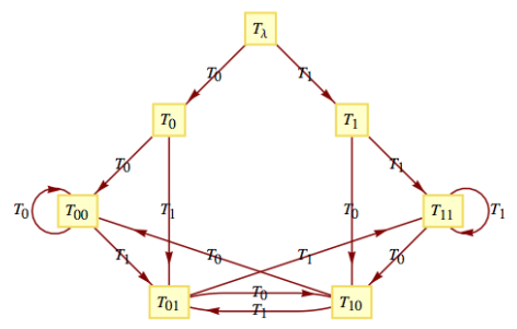
Let \(U\) be the monoid that we obtained from the unit-time delay machine (Example 14.4.2). We have seen that the machine of the monoid of the parity checker is essentially the parity checker. Will we obtain a unit-time delay machine when we construct the machine of \(U\text{?}\) We can't expect to get exactly the same machine because the unit-time delay machine is not a state machine and the machine of a monoid is a state machine. However, we will see that our new machine is capable of telling us what input was received in the previous time period. The operation table for the monoid serves as a table to define the transition function for the machine. The row headings are the state values, while the column headings are the inputs. If we were to draw a transition diagram with all possible inputs, the diagram would be too difficult to read. Since \(U\) is generated by the two elements, \(T_0\) and \(T_1\text{,}\) we will include only those inputs. Suppose that we wanted to read the transition function for the input \(T_{01}\text{.}\) Since \(T_{01}=T_0T_1\text{,}\) in any state \(s, t\left(s, T_{01}\right) = t\left(t\left(s, T_0\right), T_1\right).\) The transition diagram appears in Figure \(\PageIndex{3}\).
 Figure \(\PageIndex{3}\): Copy and Paste Caption here. (Copyright; author via source)
If we start reading a string of 0's and 1's while in state \(T_{\lambda }\) and are in state \(T_{ab}\) at any one time, the input from the previous time period (not the input that sent us into \(T_{ab}\text{,}\) the one before that) is \(a\text{.}\) In states \(T_{\lambda }, T_0\) and \(T_1\text{,}\) no previous input exists.
14.5.1: Exercises
Exercise \(\PageIndex{1}\)
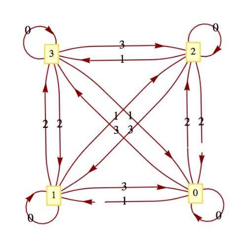
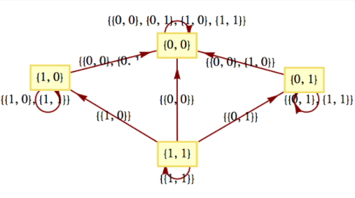
Draw the transition diagrams for the machines of the following monoids:
- \(\displaystyle \left[\mathbb{Z}_4;+_4\right]\)
- The direct product of \(\left[\mathbb{Z}_2;\times _2\right]\) with itself.
- Answer
-
 Figure \(\PageIndex{4}\): (a)
 Figure \(\PageIndex{5}\): (b)
Exercise \(\PageIndex{2}\)
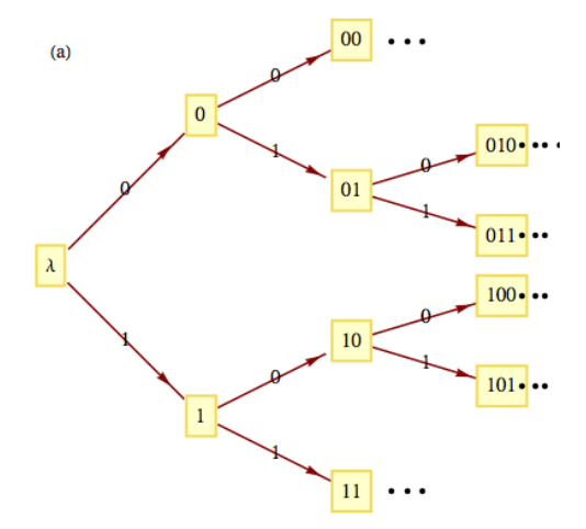
Even though a monoid may be infinite, we can visualize it as an infinite-state machine provided that it is generated by a finite number of elements. For example, the monoid \(B^*\) is generated by 0 and 1. A section of its transition diagram can be obtained by allowing input only from the generating set. The monoid of integers under addition is generated by the set \(\{-1, 1\}\text{.}\) The transition diagram for this monoid can be visualized by drawing a small portion of it, as in Figure \(\PageIndex{6}\). The same is true for the additive monoid of integers, as seen in Figure \(\PageIndex{7}\).
 Figure \(\PageIndex{6}\): An infinite machine \(B^*\)
 Figure \(\PageIndex{7}\): An infinite machine \([\mathbb{Z};+]\)
- Draw a transition diagram for \(\{a, b, c\}\)
- Draw a transition diagram for \([\mathbb{Z}\times \mathbb{Z};\textrm{componentwise addition}]\text{.}\)
- Draw a transition diagram for \([\mathbb{Z};+]\) with generating set \(\{5,-2\}\text{.}\)


