13.2: Hamilton Paths and Cycles

Last updated
Save as PDF

Page ID: 60139

Joy Morris
University of Lethbridge

$ \newcommand{\vecs}[1]{\overset { \scriptstyle \rightharpoonup} {\mathbf{#1}} } $ $ \newcommand{\vecd}[1]{\overset{-\!-\!\rightharpoonup}{\vphantom{a}\smash {#1}}} $$\newcommand{\id}{\mathrm{id}}$ $ \newcommand{\Span}{\mathrm{span}}$ $ \newcommand{\kernel}{\mathrm{null}\,}$ $ \newcommand{\range}{\mathrm{range}\,}$ $ \newcommand{\RealPart}{\mathrm{Re}}$ $ \newcommand{\ImaginaryPart}{\mathrm{Im}}$ $ \newcommand{\Argument}{\mathrm{Arg}}$ $ \newcommand{\norm}[1]{\| #1 \|}$ $ \newcommand{\inner}[2]{\langle #1, #2 \rangle}$ $ \newcommand{\Span}{\mathrm{span}}$ $\newcommand{\id}{\mathrm{id}}$ $ \newcommand{\Span}{\mathrm{span}}$ $ \newcommand{\kernel}{\mathrm{null}\,}$ $ \newcommand{\range}{\mathrm{range}\,}$ $ \newcommand{\RealPart}{\mathrm{Re}}$ $ \newcommand{\ImaginaryPart}{\mathrm{Im}}$ $ \newcommand{\Argument}{\mathrm{Arg}}$ $ \newcommand{\norm}[1]{\| #1 \|}$ $ \newcommand{\inner}[2]{\langle #1, #2 \rangle}$ $ \newcommand{\Span}{\mathrm{span}}$$\newcommand{\AA}{\unicode[.8,0]{x212B}}$

Sometimes, rather than traveled along every connection in a network, our object is simply to visit every node of the network. This relates to a different structure in the corresponding graph.

Definition: Hamilton Cycle

A Hamilton cycle is a cycle that visits every vertex of the graph. A Hamilton path is a path that visits every vertex of the graph.

The definitions of path and cycle ensure that vertices are not repeated. Hamilton paths and cycles are important tools for planning routes for tasks like package delivery, where the important point is not the routes taken, but the places that have been visited.

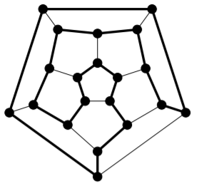
In 1857, William Rowan Hamilton first presented a game he called the “icosian game.” It involved tracing edges of a dodecahedron in such a way as to visit each corner precisely once. In fact, two years earlier Reverend Thomas Kirkman had sent a paper to the Royal Society in London, in which he posed the problem of finding what he called closed polygons in polyhedra; a closed polygon he defined as a circuit of edges that passes through each vertex just once. Thus, Kirkman had posed a more general problem prior to Hamilton (and made some progress toward solving it); nonetheless, it is Hamilton for whom these structures are now named. As we’ll see later when studying Steiner Triple Systems in design theory, Kirkman was a gifted mathematician who seems to have been singularly unlucky in terms of receiving proper credit for his achievements. As his title indicates, Kirkman was a minister who pursued mathematics on the side, as a personal passion.

Hamilton managed to convince the company of John Jacques and sons, who were manufacturers of toys (including high-quality chess sets) to produce and market the “icosian game.” It was produced under the name Around the World, and sold in two forms: a flat board, or an actual dodecahedron. In both cases, nails were placed at the corners of the dodecahedron representing cities, and the game was played by wrapping a string around the nails, traveled only along edges, visiting each nail once, and ending at the starting point. Unfortunately, the game was not a financial success. It is not very difficult and becomes uninteresting once solved.

The thick edges form a Hamilton cycle in the graph of the dodecahedron:

$clipboard_ea090fabf325d0065e6eb02dd339a1509.png$

Not every connected graph has a Hamilton cycle; in fact, not every connected graph has a Hamilton path.

Figure $\PageIndex{1}$: A graph with a Hamilton path but no Hamilton cycle. (Copyright; author via source)

Figure $\PageIndex{2}$: A graph with no Hamilton path. (Copyright; author via source)

Unfortunately, in contrast to Euler’s result about Euler tours and trails (given in Theorem 13.1.1 and Corollary 13.1.1), there is no known characterisation that enables us to quickly determine whether or not an arbitrary graph has a Hamilton cycle (or path). This is a hard problem in general. We do know of some necessary conditions (any graph that fails to meet these conditions cannot have a Hamilton cycle) and some sufficient conditions (any graph that meets these must have a Hamilton cycle). However, many graphs fail to meet any of these conditions. There are also some conditions that are either necessary or sufficient for the existence of a Hamilton path.

Here is a necessary condition for a graph to have a Hamilton cycle.

Theorem $\PageIndex{1}$

If $G$ is a graph with a Hamilton cycle, then for every $S ⊂ V$ with $S \neq ∅$, $V$, the graph $G \setminus S$ has at most $|S|$ connected components.

Proof

Let $C$ be a Hamilton cycle in $G$. Fix an arbitrary proper, nonempty subset $S$ of $V$.

One at a time, delete the vertices of $S$ from $C$. After the first vertex is deleted, the result is still connected, but has become a path. When any of the subsequent $|S| − 1$ vertices is deleted, it either breaks some path into two shorter paths (increasing the number of connected components by one) or removes a vertex at an end of some path (leaving the number of connected components unchanged, or reducing it by one if this component was a $P_0$). So $C \setminus S$ has at most $1 + (|S| − 1) = |S|$ connected components.

Notice that if two vertices $u$ and $v$ are in the same connected component of $C \setminus S$, then they will also be in the same connected component of $G \setminus S$. This is because adding edges can only connect things more fully, reducing the number of connected components. More formally, if there is a $u − v$ walk in $C$, then any pair of consecutive vertices in that walk is adjacent in $C$ so is also adjacent in $G$. Therefore the same walk is a $u − v$ walk in $G$. This tells us that the number of connected components of $G \setminus S$ is at most the number of connected components of $C \setminus S$, which we have shown to be at most $|S|$.

Example $\PageIndex{1}$

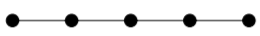
When a non-leaf is deleted from a path of length at least $2$, the deletion of this single vertex leaves two connected components. So no path of length at least $2$ contains a Hamilton cycle.

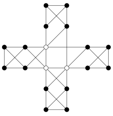
Here’s a graph in which the non-existence of a Hamilton cycle might be less obvious without Theorem 13.2.1. Deleting the three white vertices leaves four connected components.

$clipboard_e1ba37eabce3d720c11d0aa90e4522f8a.png$

As you might expect, if all of the vertices of a graph have sufficiently high valency, it will always be possible to find a Hamilton cycle in the graph. (In fact, generally the graph will have many different Hamilton cycles.) Before we can formalise this idea, it is helpful to have an additional piece of notation.

Definition: Minimum and Maximum Valency

The minimum valency of a graph $G$ is

\[\min_{v∈V}d(v).\]

The maximum valency of a graph $G$ is

\[\max_{v∈V}d(v).\]

Notation

We use $δ$ to denote the minimum valency of a graph, and $∆$ to denote its maximum valency. If we need to clarify the graph involved, we use $δ(G)$ or $∆(G)$.

Theorem $\PageIndex{2}$: (Dirac, $1952$)

If $G$ is a graph with vertex set $V$ such that $|V| ≥ 3$ and $δ(G) ≥ \dfrac{|V|}{2}$, then $G$ has a Hamilton cycle.

Proof

Towards a contradiction, suppose that $G$ is a graph with vertex set $V$, that $|V| = n ≥ 3$, and that $δ(G) ≥ \dfrac{n}{2}$, but $G$ has no Hamilton cycle.

Repeat the following as many times as possible: if there is an edge that can be added to $G$ without creating a Hamilton cycle in the resulting graph, add that edge to $G$. When this has been done as many times as possible, call the resulting graph $H$. The graph $H$ has the same vertex set $V$, and since we have added edges we have not decreased the valency of any vertex, so we have $δ(H) ≥ \dfrac{n}{2}$. Now, $H$ still has no Hamilton cycle, but adding any edge to $H$ gives a graph that does have a Hamilton cycle.

Since complete graphs on at least three vertices always have Hamilton cycles (see Exercise 13.2.1(1)), we must have $H \ncong K_n$, so there are at least two vertices of $H$, say $u$ and $v$, that are not adjacent. By our construction of $H$ from $G$, adding the edge $uv$ to $H$ would result in a Hamilton cycle, and this Hamilton cycle must use the edge $uv$ (otherwise it would be a Hamilton cycle in $H$, but $H$ has no Hamilton cycle). Thus, the portion of the Hamilton cycle that is in $H$ forms a Hamilton path from $u$ to $v$. Write this Hamilton path as

\[(u = u_1, u_2, . . . , u_n = v)\]

Define the sets

\[S = \{ui | u ∼ u_{i+1}\} \text{ and } T = {u_i | v ∼ u_i}.\]

That is, $S$ is the set of vertices that appear immediately before a neighbour of $u$ on the Hamilton path, while $T$ is the set of vertices on the Hamilton path that are neighbours of $v$. Notice that $v = u_n \notin S$ since $u_{n+1}$ isn’t defined, and $v = u_n \notin T$ since our graphs are simple (so have no loops). Thus, $u_n \notin S ∪ T$, so $|S ∪ T| < n$.

Towards a contradiction, suppose that for some $i$, $u_i ∈ S ∩ T$. Then by the definitions of $S$ and $T$, we have $u ∼ u_{i+1}$ and $v ∼ u_i$, so:

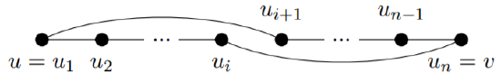
$clipboard_e00e1ef1b96a041a4e0c76f928aed1713.png$

is a Hamilton cycle in $H$, which contradicts our construction of $H$ as a graph that has no Hamilton cycle. This contradiction serves to prove that $|S ∩ T| = ∅$.

Now we have

\[d_H(u) + d_H(v) = |S| + |T| = |S ∪ T| + |S ∩ T|\]

(the last equality comes from Inclusion-Exclusion). But we have seen that $|S ∪ T| < n$ and $|S ∩ T| = 0$, so this gives

\[d_H(u) + d_H(v) < n.\]

This contradicts $δ(H) ≥ \dfrac{n}{2}$, since

\[d_H(u), d_H(v) ≥ δ(H)\]

This contradiction serves to prove that no graph $G$ with vertex set $V$ such that $|V| ≥ 3$ and $δ(G) ≥ \dfrac{|V|}{2}$ can fail to have a Hamilton cycle.

In fact, the statement of Dirac’s theorem was improved by Bondy and Chvatal in 1974. They began by observing that the proof given above for Dirac’s Theorem actually proves the following result.

Lemma $\PageIndex{1}$

Suppose that $G$ is a graph on $n$ vertices, $u$ and $v$ are nonadjacent vertices of $G$, and $d(u) + d(v) ≥ n$. Then $G$ has a Hamilton cycle if and only if the graph obtained by adding the edge $uv$ to $G$ has a Hamilton cycle.

With this in mind, they made the following definition.

Definition: Closure

Let $G$ be a graph on $n$ vertices. The closure of $G$ is the graph obtained by repeatedly joining pairs of nonadjacent vertices $u$ and $v$ for which $d(u) + d(v) ≥ n$, until no such pair exists.

Before they were able to work with this definition, they had to prove that the closure of a graph is well-defined. In other words, since there will often be choices involved in forming the closure of a graph (if more than one pair of vertices satisfy the condition, which edge do we add first?), is it possible that by making different choices, we might end up with a different graph at the end? The answer, fortunately, is no; any graph has a unique closure, as we will now prove.

Lemma $\PageIndex{2}$

Closure is well-defined. That is, any graph has a unique closure.

Proof

Let $(e_1, . . . , e_{\ell})$ be one sequence of edges we can choose to arrive at the closure of $G$, and let the resulting closure be the graph $G_1$. Let $(f_1, . . . , f_m)$ be another such sequence, and let the resulting closure be the graph $G_2$. We will prove by induction on $\ell$ that for every $1 ≤ i ≤ \ell, e_i ∈ \{f_1, . . . , f_m\}$. We will use $\{u_i , v+i\}$ to denote the endvertices of $e_i$.

Base case: $\ell = 1$, so only the edge $\{u_1, v_1\}$ is added to $G$ in order to form $G_1$. Since this was the first edge added, we must have

\[d_G(u_1) + d_G(v_1) ≥ n\]

Since $G_2$ has all of the edges of $G$, we must certainly have

\[d_{G_2} (u_1) + d_{G_2} (v_1) ≥ n.\]

Since $G_2$ is a closure of $G$, it has no pair of nonadjacent edges whose valencies sum to $n$ or higher, so $u_1$ must be adjacent to $v_1$ in $G_2$. Since the edge $u_1v_1$ was not in $G$, it must be in $\{f_1, . . . , f_m\}$. This completes the proof of the base case.

Inductive step: We begin with the inductive hypothesis. Let $k ≥ 1$ be arbitrary (with $k ≤ \ell$), and suppose that

\[e_1, . . . , e_k ∈ \{f_1, . . . , f_m\}.\]

Consider $e_{k+1} = \{u_{k+1}, v_{k+1}\}$. Let $G_0$ be the graph obtained by adding the edges $e_1, . . . , e_k$ to $G$. Since $e_{k+1}$ was chosen to add to $G_0$ to form $G_1$, it must be the case that

\[d_{G'}(u_{k+1}) + d_{G'}(v_{k+1}) ≥ n.\]

By our induction hypothesis, all of the edges of $G_0$ are also in $G_2$, so this means

\[d_{G_2}(u_{k+1}) + d_{G_2}(v_{k+1}) ≥ n.\]

Since $G_2$ is a closure of $G$, it has no pair of nonadjacent edges whose valencies sum to $n$ or higher, so $u_{k+1}$ must be adjacent to $v_{k+1}$ in $G_2$. Since the edge $e_{k+1}$ was not in $G$, it must be in $\{f_1, . . . , f_m\}$.

By the Principle of Mathematical Induction, $G_2$ contains all of the edges of $G_1$. Since there was nothing special about $G_2$ as distinct from $G_1$, we could use the same proof to show that $G_1$ contains all of the edges of $G_2$. Therefore, $G_1$ and $G_2$ have the same edges. Since they also have the same vertices (the vertices of $G$), they are the same graph. Thus, the closure of any graph is unique.

This allowed Bondy and Chvatal to deduce the following result, which is stronger than Dirac’s although as we’ve seen the proof is not significantly different.

Theorem $\PageIndex{3}$

A simple graph has a Hamilton cycle if and only if its closure has a Hamilton cycle.

Proof: Repeatedly apply Lemma 13.2.1.

This has a very nice corollary.

Corollary $\PageIndex{1}$

A simple graph on at least $3$ vertices whose closure is complete, has a Hamilton cycle.

Proof: This is an immediate consequence of Theorem 13.2.3 together with the fact (see Exercise 13.2.1(1)) that every complete graph on at least $3$ vertices has a Hamilton cycle.

Exercise $\PageIndex{1}$

1) Prove by induction that for every $n ≥ 3$, $K_n$ has a Hamilton cycle.

2) Find the closure of each of these graphs. Can you easily tell from the closure whether or not the graph has a Hamilton cycle?

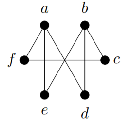
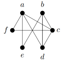
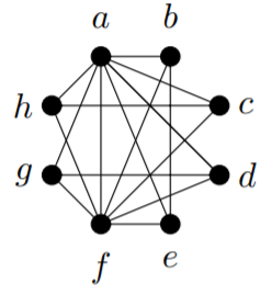
a) $clipboard_e3a43209a0e3ab890cb1dbaefb7b997bc.png$

b) $clipboard_e9f91fb4ac9a10ffb9a87ea0194077a1c.png$

3) Use Theorem 13.2.1 to prove that this graph does not have a Hamilton cycle.

$clipboard_e6c98838b1ce95db5f794d050ec560220.png$

4) Prove that if $G$ has a Hamilton path, then for every nonempty proper subset $S$ of $V$, $G − S$ has no more than $|S| + 1$ connected components.

5) For the two graphs in Exercise 13.2.1(2), either find a Hamilton cycle or use Theorem 13.2.1 to show that no Hamilton cycle exists.