5.8: Graph Coloring

Last updated
Save as PDF

Page ID: 7204

$guichard.png$
David Guichard
Professor (Mathematics) at Whitman College

$ \newcommand{\vecs}[1]{\overset { \scriptstyle \rightharpoonup} {\mathbf{#1}} } $ $ \newcommand{\vecd}[1]{\overset{-\!-\!\rightharpoonup}{\vphantom{a}\smash {#1}}} $$\newcommand{\id}{\mathrm{id}}$ $ \newcommand{\Span}{\mathrm{span}}$ $ \newcommand{\kernel}{\mathrm{null}\,}$ $ \newcommand{\range}{\mathrm{range}\,}$ $ \newcommand{\RealPart}{\mathrm{Re}}$ $ \newcommand{\ImaginaryPart}{\mathrm{Im}}$ $ \newcommand{\Argument}{\mathrm{Arg}}$ $ \newcommand{\norm}[1]{\| #1 \|}$ $ \newcommand{\inner}[2]{\langle #1, #2 \rangle}$ $ \newcommand{\Span}{\mathrm{span}}$ $\newcommand{\id}{\mathrm{id}}$ $ \newcommand{\Span}{\mathrm{span}}$ $ \newcommand{\kernel}{\mathrm{null}\,}$ $ \newcommand{\range}{\mathrm{range}\,}$ $ \newcommand{\RealPart}{\mathrm{Re}}$ $ \newcommand{\ImaginaryPart}{\mathrm{Im}}$ $ \newcommand{\Argument}{\mathrm{Arg}}$ $ \newcommand{\norm}[1]{\| #1 \|}$ $ \newcommand{\inner}[2]{\langle #1, #2 \rangle}$ $ \newcommand{\Span}{\mathrm{span}}$

As we briefly discussed in section 1.1, the most famous graph coloring problem is certainly the map coloring problem, proposed in the nineteenth century and finally solved in 1976.

Definition: A proper coloring

A proper coloring of a graph is an assignment of colors to the vertices of the graph so that no two adjacent vertices have the same color.

Usually we drop the word "proper'' unless other types of coloring are also under discussion. Of course, the "colors'' don't have to be actual colors; they can be any distinct labels—integers, for example. If a graph is not connected, each connected component can be colored independently; except where otherwise noted, we assume graphs are connected. We also assume graphs are simple in this section.

Graph coloring has many applications in addition to its intrinsic interest.

Example $\PageIndex{1}$

Example 5.8.2 If the vertices of a graph represent academic classes, and two vertices are adjacent if the corresponding classes have people in common, then a coloring of the vertices can be used to schedule class meetings. Here the colors would be schedule times, such as 8MWF, 9MWF, 11TTh, etc.

Example $\PageIndex{2}$

Example 5.8.3 If the vertices of a graph represent radio stations, and two vertices are adjacent if the stations are close enough to interfere with each other, a coloring can be used to assign non-interfering frequencies to the stations.

Example $\PageIndex{3}$

Example 5.8.4 If the vertices of a graph represent traffic signals at an intersection, and two vertices are adjacent if the corresponding signals cannot be green at the same time, a coloring can be used to designate sets of signals than can be green at the same time.

Graph coloring is closely related to the concept of an independent set.

Definition: independent

A set $S$ of vertices in a graph is independent if no two vertices of $S$ are adjacent.

If a graph is properly colored, the vertices that are assigned a particular color form an independent set. Given a graph $G$ it is easy to find a proper coloring: give every vertex a different color. Clearly the interesting quantity is the minimum number of colors required for a coloring. It is also easy to find independent sets: just pick vertices that are mutually non-adjacent. A single vertex set, for example, is independent, and usually finding larger independent sets is easy. The interesting quantity is the maximum size of an independent set.

Definition: chromatic number

The chromatic number of a graph $G$ is the minimum number of colors required in a proper coloring; it is denoted $\chi(G)$. The independence number of $G$ is the maximum size of an independent set; it is denoted $\alpha(G)$.

The natural first question about these graphical parameters is: how small or large can they be in a graph $G$ with $n$ vertices. It is easy to see that

\[\eqalign{ 1&\le \chi(G)\le n\cr 1&\le \alpha(G)\le n\cr }\]

and that the limits are all attainable: A graph with no edges has chromatic number 1 and independence number $n$, while a complete graph has chromatic number $n$ and independence number 1. These inequalities are thus not very interesting. We will see some that are more interesting.

Another natural question: What is the relation between the chromatic number of a graph $G$ and chromatic number of a subgraph of $G$? This too is simple, but quite useful at times.

Theorem 5.8.7

If $H$ is a subgraph of $G$, $\chi(H)\le \chi(G)$.

Proof

Any coloring of $G$ provides a proper coloring of $H$, simply by assigning the same colors to vertices of $H$ that they have in $G$. This means that $H$ can be colored with $\chi(G)$ colors, perhaps even fewer, which is exactly what we want.

$\square$

Often this fact is interesting "in reverse''. For example, if $G$ has a subgraph $H$ that is a complete graph $K_m$, then $\chi(H)=m$ and so $\chi(G)\ge m$. A subgraph of $G$ that is a complete graph is called a clique, and there is an associated graphical parameter.

Definition: clique number

The clique number of a graph $G$ is the largest $m$ such that $K_m$ is a subgraph of $G$.

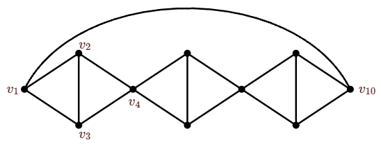
It is tempting to speculate that the only way a graph $G$ could require $m$ colors is by having such a subgraph. This is false; graphs can have high chromatic number while having low clique number; see figure 5.8.1. It is easy to see that this graph has $\chi\ge 3$, because there are many 3-cliques in the graph. In general it can be difficult to show that a graph cannot be colored with a given number of colors, but in this case it is easy to see that the graph cannot in fact be colored with three colors, because so much is "forced''. Suppose the graph can be colored with 3 colors. Starting at the left if vertex $v_1$ gets color 1, then $v_2$ and $v_3$ must be colored 2 and 3, and vertex $v_4$ must be color 1. Continuing, $v_{10}$ must be color 1, but this is not allowed, so $\chi>3$. On the other hand, since $v_{10}$ can be colored 4, we see $\chi=4$.

Paul Erdős showed in 1959 that there are graphs with arbitrarily large chromatic number and arbitrarily large girth (the girth is the size of the smallest cycle in a graph). This is much stronger than the existence of graphs with high chromatic number and low clique number.

Figure 5.8.1. A graph with clique number 3 and chromatic number 4.

Bipartite graphs with at least one edge have chromatic number 2, since the two parts are each independent sets and can be colored with a single color. Conversely, if a graph can be 2-colored, it is bipartite, since all edges connect vertices of different colors. This means it is easy to identify bipartite graphs: Color any vertex with color 1; color its neighbors color 2; continuing in this way will or will not successfully color the whole graph with 2 colors. If it fails, the graph cannot be 2-colored, since all choices for vertex colors are forced.

If a graph is properly colored, then each color class (a color class is the set of all vertices of a single color) is an independent set.

Theorem 5.8.9

In any graph $G$ on $n$ vertices, $\ds {n\over \alpha}\le\chi$.

Proof

Suppose $G$ is colored with $\chi$ colors. Since each color class is independent, the size of any color class is at most $\alpha$. Let the color classes be $V_1,V_2,\ldots,V_\chi$. Then $$ n=\sum_{i=1}^\chi |V_i| \le \chi\alpha, $$ as desired.

$\square$

We can improve the upper bound on $\chi(G)$ as well. In any graph $G$, $\Delta(G)$ is the maximum degree of any vertex.

Theorem 5.8.10

In any graph $G$, $\ds \chi\le\Delta+1$.

Proof

We show that we can always color $G$ with $\Delta+1$ colors by a simple greedy algorithm: Pick a vertex $v_n$, and list the vertices of $G$ as $v_1,v_2,\ldots,v_n$ so that if $i< j$, $\d(v_i,v_n) \ge\d(v_j,v_n)$, that is, we list the vertices farthest from $v_n$ first. We use integers $1,2,\ldots, \Delta+1$ as colors. Color $v_1$ with 1. Then for each $v_i$ in order, color $v_i$ with the smallest integer that does not violate the proper coloring requirement, that is, which is different than the colors already assigned to the neighbors of $v_i$. For $i< n$, we claim that $v_i$ is colored with one of $1,2,\ldots,\Delta$.

This is certainly true for $v_1$. For $1< i< n$, $v_i$ has at least one neighbor that is not yet colored, namely, a vertex closer to $v_n$ on a shortest path from $v_n$ to $v_i$. Thus, the neighbors of $v_i$ use at most $\Delta-1$ colors from the colors $1,2,\ldots,\Delta$, leaving at least one color from this list available for $v_i$.

Once $v_1,\ldots,v_{n-1}$ have been colored, all neighbors of $v_n$ have been colored using the colors $1,2,\ldots,\Delta$, so color $\Delta+1$ may be used to color $v_n$.

$\square$

Note that if $\d(v_n)< \Delta$, even $v_n$ may be colored with one of the colors $1,2,\ldots,\Delta$. Since the choice of $v_n$ was arbitrary, we may choose $v_n$ so that $\d(v_n)< \Delta$, unless all vertices have degree $\Delta$, that is, if $G$ is regular. Thus, we have proved somewhat more than stated, namely, that any graph $G$ that is not regular has $\chi\le\Delta$. (If instead of choosing the particular order of $v_1,\ldots,v_n$ that we used we were to list them in arbitrary order, even vertices other than $v_n$ might require use of color $\Delta+1$. This gives a slightly simpler proof of the stated theorem.) We state this as a corollary.

Corollary 5.8.11

If $G$ is not regular, $\chi\le\Delta$.

There are graphs for which $\chi=\Delta+1$: any cycle of odd length has $\Delta=2$ and $\chi=3$, and $K_n$ has $\Delta=n-1$ and $\chi=n$. Of course, these are regular graphs. It turns out that these are the only examples, that is, if $G$ is not an odd cycle or a complete graph, then $\chi(G)\le\Delta(G)$.

Theorem 5.8.12 (Brooks's Theorem)

If $G$ is a graph other than $K_n$ or $C_{2n+1}$, $\chi\le \Delta$.

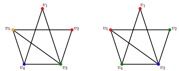
The greedy algorithm will not always color a graph with the smallest possible number of colors. Figure 5.8.2 shows a graph with chromatic number 3, but the greedy algorithm uses 4 colors if the vertices are ordered as shown.

Figure 5.8.2. A greedy coloring on the left and best coloring on the right.

In general, it is difficult to compute $\chi(G)$, that is, it takes a large amount of computation, but there is a simple algorithm for graph coloring that is not fast. Suppose that $v$ and $w$ are non-adjacent vertices in $G$. Denote by $G+\{v,w\}=G+e$ the graph formed by adding edge $e=\{v,w\}$ to $G$. Denote by $G/e$ the graph in which $v$ and $w$ are "identified'', that is, $v$ and $w$ are replaced by a single vertex $x$ adjacent to all neighbors of $v$ and $w$. (But note that we do not introduce multiple edges: if $u$ is adjacent to both $v$ and $w$ in $G$, there will be a single edge from $x$ to $u$ in $G/e$.)

Consider a proper coloring of $G$ in which $v$ and $w$ are different colors; then this is a proper coloring of $G+e$ as well. Also, any proper coloring of $G+e$ is a proper coloring of $G$ in which $v$ and $w$ have different colors. So a coloring of $G+e$ with the smallest possible number of colors is a best coloring of $G$ in which $v$ and $w$ have different colors, that is, $\chi(G+e)$ is the smallest number of colors needed to color $G$ so that $v$ and $w$ have different colors.

If $G$ is properly colored and $v$ and $w$ have the same color, then this gives a proper coloring of $G/e$, by coloring $x$ in $G/e$ with the same color used for $v$ and $w$ in $G$. Also, if $G/e$ is properly colored, this gives a proper coloring of $G$ in which $v$ and $w$ have the same color, namely, the color of $x$ in $G/e$. Thus, $\chi(G/e)$ is the smallest number of colors needed to properly color $G$ so that $v$ and $w$ are the same color.

The upshot of these observations is that $\ds\chi(G)=\min(\chi(G+e),\chi(G/e))$. This algorithm can be applied recursively, that is, if $G_1=G+e$ and $G_2=G/e$ then $\ds\chi(G_1)=\min(\chi(G_1+e),\chi(G_1/e))$ and $\ds\chi(G_2)=\min(\chi(G_2+e),\chi(G_2/e))$, where of course the edge $e$ is different in each graph. Continuing in this way, we can eventually compute $\chi(G)$, provided that eventually we end up with graphs that are "simple'' to color. Roughly speaking, because $G/e$ has fewer vertices, and $G+e$ has more edges, we must eventually end up with a complete graph along all branches of the computation. Whenever we encounter a complete graph $K_m$ it has chromatic number $m$, so no further computation is required along the corresponding branch. Let's make this more precise.

Theorem 5.8.13

The algorithm above correctly computes the chromatic number in a finite amount of time.

Proof

Suppose that a graph $G$ has $n$ vertices and $m$ edges. The number of pairs of non-adjacent vertices is $\na(G)={n\choose 2}-m$. The proof is by induction on $\na$.

If $\na(G)=0$ then $G$ is a complete graph and the algorithm terminates immediately.

Now we note that $\na(G+e)< \na(G)$ and $\na(G/e)< \na(G)$: $$ \na(G+e)={n\choose 2}-(m+1)=\na(G)-1 $$ and $$ \na(G/e)={n-1\choose 2}-(m-c), $$ where $c$ is the number of neighbors that $v$ and $w$ have in common. Then $$\eqalign{ \na(G/e)&={n-1\choose 2}-m+c\cr &\le {n-1\choose 2}-m+n-2\cr &={(n-1)(n-2)\over 2}-m+n-2\cr &={n(n-1)\over 2}-{2(n-1)\over 2}-m+n-2\cr &={n\choose 2} -m -1\cr &=\na(G)-1.\cr }\]

Now if $\na(G)>0$, $G$ is not a complete graph, so there are non-adjacent vertices $v$ and $w$. By the induction hypothesis the algorithm computes $\chi(G+e)$ and $\chi(G/e)$ correctly, and finally it computes $\chi(G)$ from these in one additional step.

$\square$

While this algorithm is very inefficient, it is sufficiently fast to be used on small graphs with the aid of a computer.

Example $\PageIndex{1}$:

Example 5.8.14

We illustrate with a very simple graph:

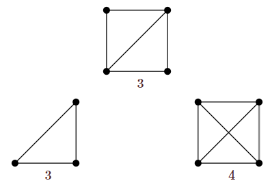
The chromatic number of the graph at the top is $\min(3,4)=3$. (Of course, this is quite easy to see directly.)

Contributors and Attributions

David Guichard (Whitman College)