
17.4: Graphing Relations
- Page ID
- 83492

Recall that if \(R\) is a relation on a set \(A\text{,}\) then formally \(R\) is a subset \(A \times A\text{.}\) In other words, \(R\) is a collection of ordered pairs of elements from \(A\text{.}\)
Also recall that in a directed graph, the edge collection is formally defined to be a collection of ordered pairs of vertices. So when the set \(A\) is finite, we may regard \(A\) as a set of vertices and \(R\) as a collection of (directed) edges in a graph!
To summarize, we may represent a relation \(R \subseteq A \times A\) by the directed graph \((A,R)\text{.}\) The vertices of the graph are the elements of \(A\text{,}\) and for elements \(a_1,a_2 \in A\text{,}\) we draw an arrow from \(a_1\) to \(a_2\) if \(a_1 \mathrel{R} a_2\) is true.
Recall that for natural numbers \(m\) and \(n\text{,}\) \(m \mid n\) means “\(m\) divides \(n\)”. Consider this relation on the finite set \(A = \{ 2,3,4,5,6,7,8,9,10 \}\text{.}\) The graph of this relation appears in Figure \(\PageIndex{1}\).
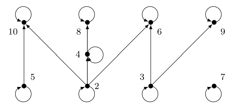
Note that each vertex has a loop since every number divides itself.
Using the same division relation on the same set \(A\) as in Example \(\PageIndex{1}\) above, we may obtain the graph for the inverse relation by just reversing the direction of all the arrows in the graph in Figure \(\PageIndex{1}\).
How are the properties of a relation reflected in its graph?
Reflexive relations.
In this case, \(a \mathrel{R} a\) is true for every element \(a \in A\text{,}\) so every vertex has a loop. For example, the relation in Example \(\PageIndex{1}\) is reflexive, and we see this mirrored in the graph in Figure \(\PageIndex{1}\) by the placement of a loop at every node.
When a relation is understood to be reflexive, we often omit the loops from its graph to reduce visual clutter.
Symmetric relations.
In this case, the conditional \(a_1 \mathrel{R} a_2 \Rightarrow a_2 \mathrel{R} a_1\) is always true. Therefore, in the graph for \(R\text{,}\) whenever we have an arrow from \(a_1\) to \(a_2\text{,}\) we must also have an arrow from \(a_2\) to \(a_1\text{.}\)
On the set \(A = \{a,b,c,d\}\text{,}\) the relation
\begin{equation*} R = \{(a,b),(b,a),(b,c),(c,b)\} \end{equation*}
is symmetric, and we see this property reflected in the graph in Figure \(\PageIndex{2}\), as each pair of related (distinct) nodes has an arrow in each direction between them.
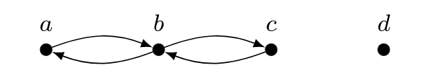 Figure \(\PageIndex{2}\): The graph of a basic symmetric relation.
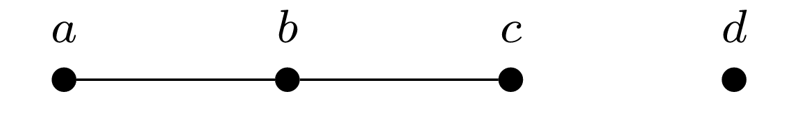
When \(R\) is symmetric, arrows are essentially meaningless since between every pair of vertices we will have either no arrows or one arrow in each direction. So we may as well draw the graph for \(R\) as an ordinary (undirected) graph instead of a directed graph, replacing each pair of arrows with a single edge.
The relation in the previous example is more concisely depicted graphically as in Figure \(\PageIndex{3}\) below.
Antisymmetric relations.
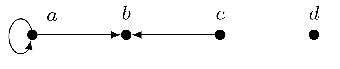
In this case, we never have both \(a_1 \mathrel{R} a_2\) and \(a_2 \mathrel{R} a_1\) for \(a_1 \ne a_2\text{,}\) so in the graph for \(R\text{,}\) no pair of vertices can have two oppositely-directed arrows between them.
On the set \(A = \{a,b,c,d\}\text{,}\) the relation
\begin{equation*} R = \{(a,a),(a,b),(c,b)\} \end{equation*}
is antisymmetric, and we see this property reflected in the graph in Figure \(\PageIndex{4}\), as each pair of distinct nodes has at most one arrow between them.
Transitive relations.
In this case, the conditional \(a_1 \mathrel{R} a_2 \land a_2 \mathrel{R} a_3 \Rightarrow a_1 \mathrel{R} a_3\) is always true. Therefore, in the graph for \(R\text{,}\) every “chain” of two arrows has a corresponding “composite” arrow.
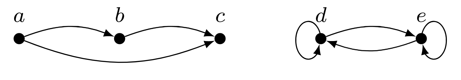
On the set \(A = \{a,b,c,d,e\} \text{,}\) the relation
\begin{equation*} R = \{(a,b),(b,c),(a,c),(d,e),(e,d),(d,d),(e,e)\} \end{equation*}
is transitive, and we see this property reflected in the graph in Figure \(\PageIndex{5}\), as each pair of arrows forming a “chain” between three nodes has a corresponding “composite” arrow from the first node in the chain to the third.
In the graph of a transitive relation, we often omit the “composite” arrows to reduce visual clutter, as we can infer from “chains” of arrows where the “composite” arrows would go. For example, we did this in both the power set graph in Example 14.4.1 (see Figure 14.4.1) and in the division graph in Example 14.4.2 (see Figure 14.4.2). It should be obvious that the relations “is a subset of” and “divides” are transitive, so there was no need to clutter up the graphs of those relations with extra “composite” arrows — we could trace the fact that one set was a subset of another or the fact that one number divides another by following a chain of arrows through intermediate nodes, as necessary.