
1.4: Other First Order Equations
- Page ID
- 91049

There are several nonlinear first order equations whose solution can be obtained using special techniques. We conclude this chapter by looking at a few of these equations named after famous mathematicians of the \(17-18\) th century inspired by various applications.
Bernoulli Equation
The Bernoulli’s were a family of Swiss mathematicians spanning three generations. It all started with Jacob Bernoulli (1654-1705) and his brother Johann Bernoulli (1667-1748). Jacob had a son, Nicolaus Bernoulli (1687- 1759) and Johann (1667-1748) had three sons, Nicolaus Bernoulli II (1695-1726), Daniel Bernoulli (1700-1872), and Johann Bernoulli II (1710-1790). The last generation consisted of Johann II’s sons, Johann Bernoulli III (1747-1807) and Jacob Bernoulli II (1759-1789). Johann, Jacob and Daniel Bernoulli were the most famous of the Bernoulli’s. Jacob studied with Leibniz, Johann studied under his older brother and later taught Leonhard Euler (1707-1783) and Daniel Bernoulli, who is known for his work in hydrodynamics.
We begin with the Bernoulli equation, named after Jacob Bernoulli (1655-1705). The Bernoulli equation is of the form
\(\dfrac{d y}{d x}+p(x) y=q(x) y^{n}, \quad n \neq 0,1\)
Note that when \(n=0,1\) the equation is linear and can be solved using an integrating factor. The key to solving this equation is using the transforma \(z(x)=\dfrac{1}{y^{n-1}(x)}\) to make the equation for \(z(x)\) linear. We demonstrate the procedure using an example.
Solve the Bernoulli equation \(x y^{\prime}+y=y^{2} \ln x\) for \(x>0\). In this example \(p(x)=1, q(x)=\ln x\), and \(n=2\). Therefore, we let mous of the Bernoulli’s. Jacob studied \(z=\dfrac{1}{y} .\) Then,
\(z^{\prime}=-\dfrac{1}{y^{2}} y^{\prime}=z^{2} y^{\prime} .\)
Inserting \(z=y^{-1}\) and \(z^{\prime}=z^{2} y^{\prime}\) into the differential equation, we have
\[ \begin{aligned} x y^{\prime}+y &=y^{2} \ln x \\ -x \dfrac{z^{\prime}}{z^{2}}+\dfrac{1}{z} &=\dfrac{\ln x}{z^{2}} \\ -x z^{\prime}+z &=\ln x \\ z^{\prime}-\dfrac{1}{x} z=-\dfrac{\ln x}{x} . \end{aligned} \end{equation}\label{1.47} \]
Thus, the resulting equation is a linear first order differential equation. It can be solved using the integrating factor,
\(\mu(x)=\exp \left(-\int \dfrac{d x}{x}\right)=\dfrac{1}{x}\)
Multiplying the differential equation by the integrating factor, we have
\(\left(\dfrac{z}{x}\right)^{\prime}=\dfrac{\ln x}{x^{2}}\)
Integrating, we obtain
\[ \begin{aligned} \dfrac{z}{x} &=-\int \dfrac{\ln x}{x^{2}}+C \\ &=\dfrac{\ln x}{x}+\int \dfrac{d x}{x^{2}}+C \\ &=\dfrac{\ln x}{x}+\dfrac{1}{x}+C \end{aligned}\label{1.48} \]
Multiplying by \(x\), we have \(z=\ln x+1+C x .\) Since \(z=y^{-1}\), the general solution to the problem is
\(y=\dfrac{1}{\ln x+1+C x}\)
Lagrange and Clairaut Equations
ALEXIS CLAUDE CLAIRAUT (1713-1765) SOLVED the differential equation
\(y=x y^{\prime}+g\left(y^{\prime}\right)\)
This is a special case of the family of Lagrange equations,
\(y=x f\left(y^{\prime}\right)+g\left(y^{\prime}\right)\)
named after Joseph Louis Lagrange (1736-1813). These equations also have solutions called singular solutions. Singular solution are solutions for which there is a failure of uniqueness to the initial value problem at every point on the curve. A singular solution is often one that is tangent to every solution in a family of solutions.
First, we consider solving the more general Lagrange equation. Let \(p=y^{\prime}\) in the Lagrange equation, giving
\[y=x f(p)+g(p) \nonumber \]
Next, we differentiate with respect to \(x\) to find
\(y^{\prime}=p=f(p)+x f^{\prime}(p) p^{\prime}+g^{\prime}(p) p^{\prime}\)
Lagrange equations, \(y=x f\left(y^{\prime}\right)+g\left(y^{\prime}\right)\).
Here we used the Chain Rule. For example,
\(\dfrac{d g(p)}{d x}=\dfrac{d g}{d p} \dfrac{d p}{d x}\)
Solving for \(p^{\prime}\), we have
\[\dfrac{d p}{d x}=\dfrac{p-f(p)}{x f^{\prime}(p)+g^{\prime}(p)} \nonumber \]
We have introduced \(p=p(x)\), viewed as a function of \(x\). Let’s assume that we can invert this function to find \(x=x(p)\). Then, from introductory calculus, we know that the derivatives of a function and its inverse are related,
\(\dfrac{d x}{d p}=\dfrac{1}{\dfrac{d p}{d x}}\)
Applying this to Equation \(\PageIndex{4}\), we have
\[ \begin{aligned} \dfrac{d x}{d p} &=\dfrac{x f^{\prime}(p)+g^{\prime}(p)}{p-f(p)} \\ x^{\prime}-\dfrac{f^{\prime}(p)}{p-f(p)} x &=\dfrac{g^{\prime}(p)}{p-f(p)} \end{aligned} \label{1.51} \]
assuming that \(p-f(p) \neq 0\).
As can be seen, we have transformed the Lagrange equation into a first order linear differential equation \(\PageIndex{5}\) for \(x(p)\). Using methods from earlier in the chapter, we can in principle obtain a family of solutions
\(x=F(p, C)\)
where \(C\) is an arbitrary integration constant. Using Equation \(\PageIndex{3}\), one might be able to eliminate \(p\) in Equation \(\PageIndex{5}\) to obtain a family of solutions of the Lagrange equation in the form
\(\varphi(x, y, C)=0\)
If it is not possible to eliminate \(p\) from Equations \(\PageIndex{3}\) and \(\PageIndex{5}\), then one could report the family of solutions as a parametric family of solutions with \(p\) the parameter. So, the parametric solutions would take the form
\[ \begin{aligned} &x=F(p, C) \\ &y=F(p, C) f(p)+g(p) \end{aligned} \label{1.52} \]
Singular solutions are possible for Lagrange equations.
We had also assumed the \(p-f(p) \neq 0\). However, there might also be solutions of Lagrange’s equation for which \(p-f(p)=0 .\) Such solutions are called singular solutions.
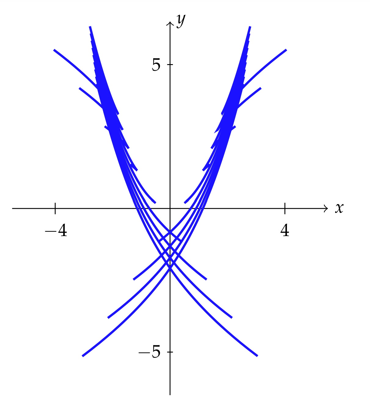
Solve the Lagrange equation \(y=2 x y^{\prime}-y^{\prime 2}\).
We will start with Equation \(\PageIndex{5}\). Noting that \(f(p)=2 p, g(p)=\) \(-p^{2}\), we have
\[ \begin{aligned}
x^{\prime}-\dfrac{f^{\prime}(p)}{p-f(p)} x &=\dfrac{g^{\prime}(p)}{p-f(p)} \\
x^{\prime}-\dfrac{2}{p-2 p} x &=\dfrac{-2 p}{p-2 p} \\
x^{\prime}+\dfrac{2}{p} x &=2 .
\end{aligned} \label{1.53} \]
This first order linear differential equation can be solved using an integrating factor. Namely,
\(\mu(p)=\exp \left(\int \dfrac{2}{p} dp\right)=e^{2 \ln p}=p^{2}\)
Multiplying the differential equation by the integrating factor, we have
\(\dfrac{d}{d p}\left(x p^{2}\right)=2 p^{2}\)
Integrating,
\(x p^{2}=\dfrac{2}{3} p^{3}+C.\)
This gives the general solution
\(x(p)=\dfrac{2}{3} p+\dfrac{C}{p^{2}}\)
Replacing \(y^{\prime}=p\) in the original differential equation, we have \(y=2 x p-p^{2}\). The family of solutions is then given by the parametric equations
\[\begin{aligned} x &=\dfrac{2}{3} p+\dfrac{C}{p^{2}}, \\ y &=2\left(\dfrac{2}{3} p+\dfrac{C}{p^{2}}\right) p-p^{2} \\ &=\dfrac{1}{3} p^{2}+\dfrac{2 C}{p} . \end{aligned} \label{1.54} \]
The plots of these solutions is shown in Figure \(\PageIndex{1}\).
We also need to check for a singular solution. We solve the equation \(p-f(p)=0\), or \(p=0 .\) This gives the solution \(y(x)=\left(2 x p-p^{2}\right) p=0=0 .\)
The Clairaut differential equation is given by
\(y=x y^{\prime}+g\left(y^{\prime}\right)\)
Letting \(p=y^{\prime}\), we have
\(y=x p+g(p)\)
This is the Lagrange equation with \(f(p)=p\). Differentiating with respect to x,
Clairaut equations, \(y=x y^{\prime}+g\left(y^{\prime}\right)\).
\(p=p+x p^{\prime}+g^{\prime}(p) p^{\prime}\)
Rearranging, we find
\(x=-g^{\prime}(p)\)
So, we have the parametric solution
\[ \begin{aligned} &x=-g^{\prime}(p) \\ &y=-p g^{\prime}(p)+g(p) \end{aligned} \label{1.55} \]
For the case that \(y^{\prime}=C\), it can be seen that \(y=C x+g(C)\) is a general solution solution.
Find the solutions of \(y=x y^{\prime}-y^{\prime 2}\).
As noted, there is a family of straight line solutions \(y=C x-C^{2}\), since \(g(p)=-p^{2}\). There might also by a parametric solution not contained \(n\) this family. It would be given by the set of equations
\[ \begin{aligned} &x=-g^{\prime}(p)=2 p \\ &y=-p g^{\prime}(p)+g(p)=2 p^{2}-p^{2}=p^{2} \end{aligned} \label{1.56} \]
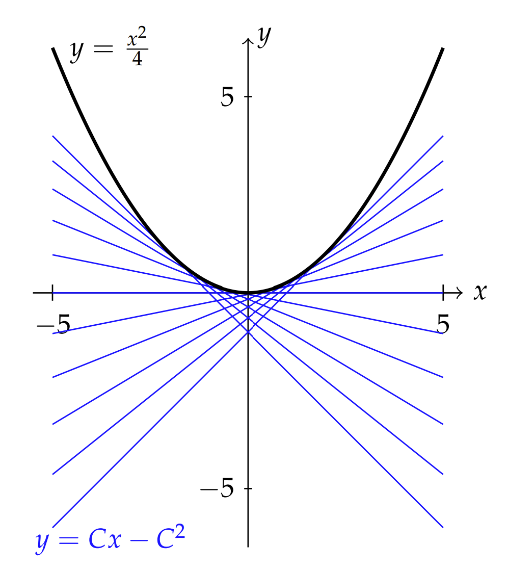
Eliminating \(p\), we have the parabolic curve \(y=x^{2} / 4\).
In Figure \(\PageIndex{2}\) we plot these solutions. The family of straight line
lutions are shown in blue. The limiting curve traced out, much like string figures one might create, is the parametric curve.
Riccati Equation
JACOPO FRANCESCO RICCATI ( \(1676-1754\) ) STUDIED CURVES With sOme specified curvature. He proposed an equation of the form
\(y^{\prime}+a(x) y^{2}+b(x) y+c(x)=0\)
around 1720. He communicated this to the Bernoulli’s. It was Daniel Bernoulli who had actually solved this equation. As noted by Ranjan Roy \((2011)\), Riccati had published his equation in 1722 with a note that D. Bernoulli giving the solution in terms of an anagram. Furthermore, when \(a \equiv 0\), the Riccati equation reduces to a Bernoulli equation.
In Section 7.2, we will show that the Ricatti equation can be transformed into a second order linear differential equation. However, there are special cases in which we can get our hands on the solutions. For example, if \(a, b\), and \(c\) are constants, then the differential equation can be integrated directly. We have
\(\dfrac{d y}{d x}=-\left(a y^{2}+b y+c\right)\)
This equation is separable and we obtain
\(x-C=-\int \dfrac{d y}{a y^{2}+b y+c}\)
When a differential equation is left in this form, it is said to be solved by quadrature when the resulting integral in principle can be computed in terms of elementary functions. \({ }^{1}\)
- 1
-
By elementary functions we mean
\[x-C=-\int \dfrac{d y}{a y^{2}+b y+c} \nonumber \]
well known functions like polynomials, trigonometric, hyperbolic, and some not so well know to undergraduates, such as Jacobi or Weierstrass elliptic functions.
If a particular solution is known, then one can obtain a solution to the Riccati equation. Let the known solution be \(y_{1}(x)\) and assume that the general solution takes the form \(y(x)=y_{1}(x)+z(x)\) for some unknown function \(z(x)\). Substituting this form into the differential equation, we can show that \(v(x)=1 / z(x)\) satisfies a first order linear differential equation.
Inserting \(y=y_{1}+z\) into the general Riccati equation, we have
\[\begin{equation} \begin{aligned} 0=& \dfrac{d y}{d x}+a(x) y^{2}+b(x) y+c \\ =& \dfrac{d z}{d x}+a z^{2}+2 a z y_{1}+b z+\\ &+\dfrac{d y_{1}}{d x}+a y_{1}^{2}+b y_{1}+c \\ =& \dfrac{d z}{d x}+a(x)\left[2 y_{1} z+z^{2}\right]+b(x) z \\ -a(x) z^{2}=& \dfrac{d z}{d x}+\left[2 a(x) y_{1}+b(x)\right] z . \end{aligned}\end{equation}\label{1.57} \]
The last equation is a Bernoulli equation with \(n=2 .\) So, we can make it a linear equation with the substitution \(z=\dfrac{1}{v}, z^{\prime}=-\dfrac{z^{\prime}}{v^{2}}\). Then, we obtain a differential equation for \(v(x)\). It is given by
\(v^{\prime}-\left(2 a(x) y_{1}(x)+b(x)\right) v=a(x)\)
Find the general solution of the Riccati equation, \(y^{\prime}-\) \(y^{2}+2 e^{x} y-e^{2 x}-e^{x}=0\), using the particular solution \(y_{1}(x)=e^{x} .\)
We let the sought solution take the form \(y(x)=z(x)+e^{x}\). Then, the equation for \(z(x)\) is found as
\(\dfrac{d z}{d x}=z^{2}\)
This equation is simple enough to integrate directly to obtain \(z=\dfrac{1}{C-x}\). Then, the solution to the problem becomes
\(y(x)=\dfrac{1}{C-x}+e^{x}\)