
4.1: Introduction to Power Series
- Page ID
- 91063

\( \newcommand{\vecs}[1]{\overset { \scriptstyle \rightharpoonup} {\mathbf{#1}} } \)
\( \newcommand{\vecd}[1]{\overset{-\!-\!\rightharpoonup}{\vphantom{a}\smash {#1}}} \)
\( \newcommand{\dsum}{\displaystyle\sum\limits} \)
\( \newcommand{\dint}{\displaystyle\int\limits} \)
\( \newcommand{\dlim}{\displaystyle\lim\limits} \)
\( \newcommand{\id}{\mathrm{id}}\) \( \newcommand{\Span}{\mathrm{span}}\)
( \newcommand{\kernel}{\mathrm{null}\,}\) \( \newcommand{\range}{\mathrm{range}\,}\)
\( \newcommand{\RealPart}{\mathrm{Re}}\) \( \newcommand{\ImaginaryPart}{\mathrm{Im}}\)
\( \newcommand{\Argument}{\mathrm{Arg}}\) \( \newcommand{\norm}[1]{\| #1 \|}\)
\( \newcommand{\inner}[2]{\langle #1, #2 \rangle}\)
\( \newcommand{\Span}{\mathrm{span}}\)
\( \newcommand{\id}{\mathrm{id}}\)
\( \newcommand{\Span}{\mathrm{span}}\)
\( \newcommand{\kernel}{\mathrm{null}\,}\)
\( \newcommand{\range}{\mathrm{range}\,}\)
\( \newcommand{\RealPart}{\mathrm{Re}}\)
\( \newcommand{\ImaginaryPart}{\mathrm{Im}}\)
\( \newcommand{\Argument}{\mathrm{Arg}}\)
\( \newcommand{\norm}[1]{\| #1 \|}\)
\( \newcommand{\inner}[2]{\langle #1, #2 \rangle}\)
\( \newcommand{\Span}{\mathrm{span}}\) \( \newcommand{\AA}{\unicode[.8,0]{x212B}}\)
\( \newcommand{\vectorA}[1]{\vec{#1}} % arrow\)
\( \newcommand{\vectorAt}[1]{\vec{\text{#1}}} % arrow\)
\( \newcommand{\vectorB}[1]{\overset { \scriptstyle \rightharpoonup} {\mathbf{#1}} } \)
\( \newcommand{\vectorC}[1]{\textbf{#1}} \)
\( \newcommand{\vectorD}[1]{\overrightarrow{#1}} \)
\( \newcommand{\vectorDt}[1]{\overrightarrow{\text{#1}}} \)
\( \newcommand{\vectE}[1]{\overset{-\!-\!\rightharpoonup}{\vphantom{a}\smash{\mathbf {#1}}}} \)
\( \newcommand{\vecs}[1]{\overset { \scriptstyle \rightharpoonup} {\mathbf{#1}} } \)
\(\newcommand{\longvect}{\overrightarrow}\)
\( \newcommand{\vecd}[1]{\overset{-\!-\!\rightharpoonup}{\vphantom{a}\smash {#1}}} \)
\(\newcommand{\avec}{\mathbf a}\) \(\newcommand{\bvec}{\mathbf b}\) \(\newcommand{\cvec}{\mathbf c}\) \(\newcommand{\dvec}{\mathbf d}\) \(\newcommand{\dtil}{\widetilde{\mathbf d}}\) \(\newcommand{\evec}{\mathbf e}\) \(\newcommand{\fvec}{\mathbf f}\) \(\newcommand{\nvec}{\mathbf n}\) \(\newcommand{\pvec}{\mathbf p}\) \(\newcommand{\qvec}{\mathbf q}\) \(\newcommand{\svec}{\mathbf s}\) \(\newcommand{\tvec}{\mathbf t}\) \(\newcommand{\uvec}{\mathbf u}\) \(\newcommand{\vvec}{\mathbf v}\) \(\newcommand{\wvec}{\mathbf w}\) \(\newcommand{\xvec}{\mathbf x}\) \(\newcommand{\yvec}{\mathbf y}\) \(\newcommand{\zvec}{\mathbf z}\) \(\newcommand{\rvec}{\mathbf r}\) \(\newcommand{\mvec}{\mathbf m}\) \(\newcommand{\zerovec}{\mathbf 0}\) \(\newcommand{\onevec}{\mathbf 1}\) \(\newcommand{\real}{\mathbb R}\) \(\newcommand{\twovec}[2]{\left[\begin{array}{r}#1 \\ #2 \end{array}\right]}\) \(\newcommand{\ctwovec}[2]{\left[\begin{array}{c}#1 \\ #2 \end{array}\right]}\) \(\newcommand{\threevec}[3]{\left[\begin{array}{r}#1 \\ #2 \\ #3 \end{array}\right]}\) \(\newcommand{\cthreevec}[3]{\left[\begin{array}{c}#1 \\ #2 \\ #3 \end{array}\right]}\) \(\newcommand{\fourvec}[4]{\left[\begin{array}{r}#1 \\ #2 \\ #3 \\ #4 \end{array}\right]}\) \(\newcommand{\cfourvec}[4]{\left[\begin{array}{c}#1 \\ #2 \\ #3 \\ #4 \end{array}\right]}\) \(\newcommand{\fivevec}[5]{\left[\begin{array}{r}#1 \\ #2 \\ #3 \\ #4 \\ #5 \\ \end{array}\right]}\) \(\newcommand{\cfivevec}[5]{\left[\begin{array}{c}#1 \\ #2 \\ #3 \\ #4 \\ #5 \\ \end{array}\right]}\) \(\newcommand{\mattwo}[4]{\left[\begin{array}{rr}#1 \amp #2 \\ #3 \amp #4 \\ \end{array}\right]}\) \(\newcommand{\laspan}[1]{\text{Span}\{#1\}}\) \(\newcommand{\bcal}{\cal B}\) \(\newcommand{\ccal}{\cal C}\) \(\newcommand{\scal}{\cal S}\) \(\newcommand{\wcal}{\cal W}\) \(\newcommand{\ecal}{\cal E}\) \(\newcommand{\coords}[2]{\left\{#1\right\}_{#2}}\) \(\newcommand{\gray}[1]{\color{gray}{#1}}\) \(\newcommand{\lgray}[1]{\color{lightgray}{#1}}\) \(\newcommand{\rank}{\operatorname{rank}}\) \(\newcommand{\row}{\text{Row}}\) \(\newcommand{\col}{\text{Col}}\) \(\renewcommand{\row}{\text{Row}}\) \(\newcommand{\nul}{\text{Nul}}\) \(\newcommand{\var}{\text{Var}}\) \(\newcommand{\corr}{\text{corr}}\) \(\newcommand{\len}[1]{\left|#1\right|}\) \(\newcommand{\bbar}{\overline{\bvec}}\) \(\newcommand{\bhat}{\widehat{\bvec}}\) \(\newcommand{\bperp}{\bvec^\perp}\) \(\newcommand{\xhat}{\widehat{\xvec}}\) \(\newcommand{\vhat}{\widehat{\vvec}}\) \(\newcommand{\uhat}{\widehat{\uvec}}\) \(\newcommand{\what}{\widehat{\wvec}}\) \(\newcommand{\Sighat}{\widehat{\Sigma}}\) \(\newcommand{\lt}{<}\) \(\newcommand{\gt}{>}\) \(\newcommand{\amp}{&}\) \(\definecolor{fillinmathshade}{gray}{0.9}\)As NOTED A FEW TIMES, not all differential equations have exact solutions. So, we need to resort to seeking approximate solutions, or solutions i the neighborhood of the initial value. Before describing these methods, we need to recall power series. A power series expansion about \(x=a\) with coefficient sequence \(c_{n}\) is given by \(\sum_{n=0}^{\infty} c_{n}(x-a)^{n}\). For now we will consider all constants to be real numbers with \(x\) in some subset of the set of real numbers. We review power series in the appendix.
The two types of series encountered in calculus are Taylor and Maclaurin series. A Taylor series expansion of \(f(x)\) about \(x=a\) is the series
(Taylor series expansion.)
\[f(x) \sim \sum_{n=0}^{\infty} c_{n}(x-a)^{n} \nonumber \]
where
\[c_{n}=\dfrac{f^{(n)}(a)}{n !} . \nonumber \]
Note that we use \(\sim\) to indicate that we have yet to determine when the series may converge to the given function.
(Maclaurin series expansion.) A Maclaurin series expansion of \(f(x)\) is a Taylor series expansion of \(f(x)\) about \(x=0\), or
\[f(x) \sim \sum_{n=0}^{\infty} c_{n} x^{n} \nonumber \]
where
\[c_{n}=\dfrac{f^{(n)}(0)}{n !} \nonumber \]
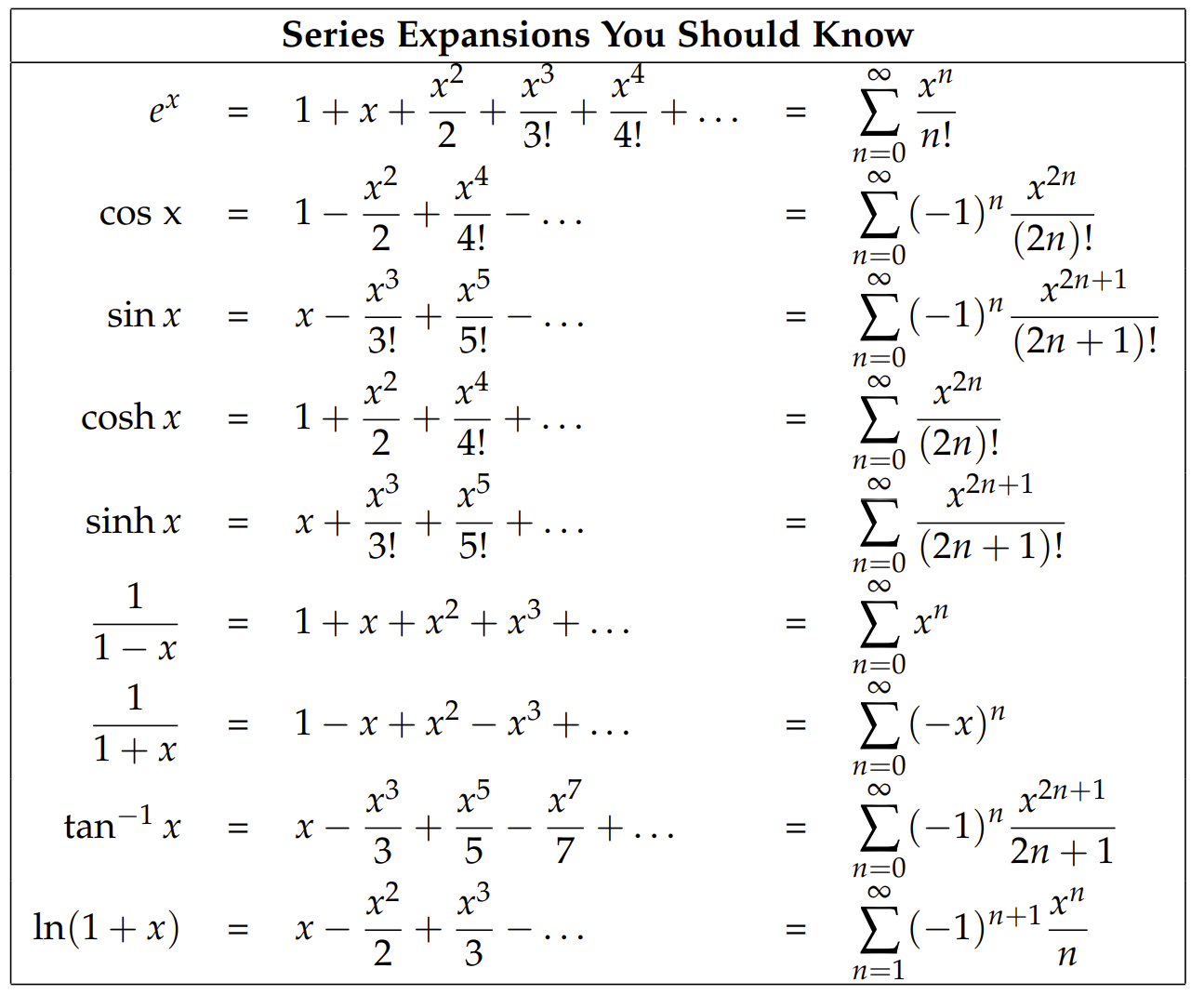
We note that Maclaurin series are a special case of Taylor series for which We note that Maclaurin series are a special case of Taylor series for which the expansion is about \(x=0 \). Typical Maclaurin series, which you should know, are given in Figure \(\PageIndex{1}\).
A simple example of developing a series solution for a differential equation is given in the next example.
\(y^{\prime}(x)=x+y(x), y(0)=1\).
We are interested in seeking solutions of this initial value problem. We note that this was already solved in Example 3.1. Let’s assume that we can write the solution as the Maclaurin series
\[\begin{equation} \begin{aligned} y(x) &=\sum_{n=0}^{\infty} \dfrac{y^{(n)}(x)}{n !} x^{n} \\[4pt] &=y(0)+y^{\prime}(0) x+\dfrac{1}{2} y^{\prime \prime}(0) x^{2}+\dfrac{1}{6} y^{\prime \prime \prime}(0) x^{3}+\ldots \end{aligned}\end{equation} \label{4.5} \]
We already know that \(y(0)=1 \). So, we know the first term in the series expansion. We can find the value of \(y^{\prime}(0)\) from the differential equation:
\[y^{\prime}(0)=0+y(0)=1 \nonumber \]
In order to obtain values of the higher order derivatives at \(x=0\), we differentiate the differential equation several times:
\[ \begin{aligned} y^{\prime \prime}(x) &=1+y^{\prime}(x) \\[4pt] y^{\prime \prime}(0) &=1+y^{\prime}(0)=2 \\[4pt] y^{\prime \prime \prime}(x) &=y^{\prime \prime}(x)=2 \end{aligned} \label{4.6} \]
All other values of the derivatives are the same. Therefore, we have
\[y(x)=1+x+2\left(\dfrac{1}{2} x^{2}+\dfrac{1}{3 !} x^{3}+\ldots\right) \nonumber. \nonumber \]
This solution can be summed as
\[y(x)=2\left(1+x+\dfrac{1}{2} x^{2}+\dfrac{1}{3 !} x^{3}+\ldots\right)-1-x=2 e^{x}-x-1 .\nonumber \]
This is the same result we had obtained before.