5.1: The Laplace Transform

Up to this point we have only explored Fourier exponential transforms as one type of integral transform. The Fourier transform is useful on infinite domains. However, students are often introduced to another integral transform, called the Laplace transform, in their introductory differential equations class. These transforms are defined over semi-infinite domains and are useful for solving initial value problems for ordinary differential equations.

The Laplace transform is named after Pierre-Simon de Laplace (1749 - 1827). Laplace made major contributions, especially to celestial mechanics, tidal analysis, and probability.

Integral transform on \([a, b]\) with respect to the integral kernel, \(K(x, k)\).

The Fourier and Laplace transforms are examples of a broader class of transforms known as integral transforms. For a function \(f(x)\) defined on an interval \((a, b)\), we define the integral transform

\[F(k)=\int_{a}^{b} K(x, k) f(x) d x\nonumber \]

where \(K(x, k)\) is a specified kernel of the transform. Looking at the Fourier transform, we see that the interval is stretched over the entire real axis and the kernel is of the form, \(K(x, k)=e^{i k x}\). In Table 5.1 we show several types of integral transforms.

Table \(\PageIndex{1}\): A Table of Common Integral Transforms.

Laplace Transform	\(F(s)=\int_{0}^{\infty} e^{-s x} f(x) d x\)
Fourier Transform	\(F(k)=\int_{-\infty}^{\infty} e^{i k x} f(x) d x\)
Fourier Cosine Transform	\(F(k)=\int_{0}^{\infty} \cos (k x) f(x) d x\)
Fourier Sine Transform	\(F(k)=\int_{0}^{\infty} \sin (k x) f(x) d x\)
Mellin Transform	\(F(k)=\int_{0}^{\infty} x^{k-1} f(x) d x\)
Hankel Transform	\(F(k)=\int_{0}^{\infty} x J_{n}(k x) f(x) d x\)

It should be noted that these integral transforms inherit the linearity of integration. Namely, let \(h(x)=\alpha f(x)+\beta g(x)\), where \(\alpha\) and \(\beta\) are constants. Then,

\[\begin{aligned} H(k) &=\int_{a}^{b} K(x, k) h(x) d x \\ &=\int_{a}^{b} K(x, k)(\alpha f(x)+\beta g(x)) d x \\ &=\alpha \int_{a}^{b} K(x, k) f(x) d x+\beta \int_{a}^{b} K(x, k) g(x) d x \\ &=\alpha F(x)+\beta G(x) \end{aligned} \label{5.1} \]

Therefore, we have shown linearity of the integral transforms. We have seen the linearity property used for Fourier transforms and we will use linearity in the study of Laplace transforms.

The Laplace transform of \(f, F=\mathcal{L}[f]\). We now turn to Laplace transforms. The Laplace transform of a function \(f(t)\) is defined as

\[F(s)=\mathcal{L}[f](s)=\int_{0}^{\infty} f(t) e^{-s t} d t, \quad s>0 \nonumber \]

This is an improper integral and one needs

\[\lim _{t \rightarrow \infty} f(t) e^{-s t}=0 \nonumber \]

to guarantee convergence.

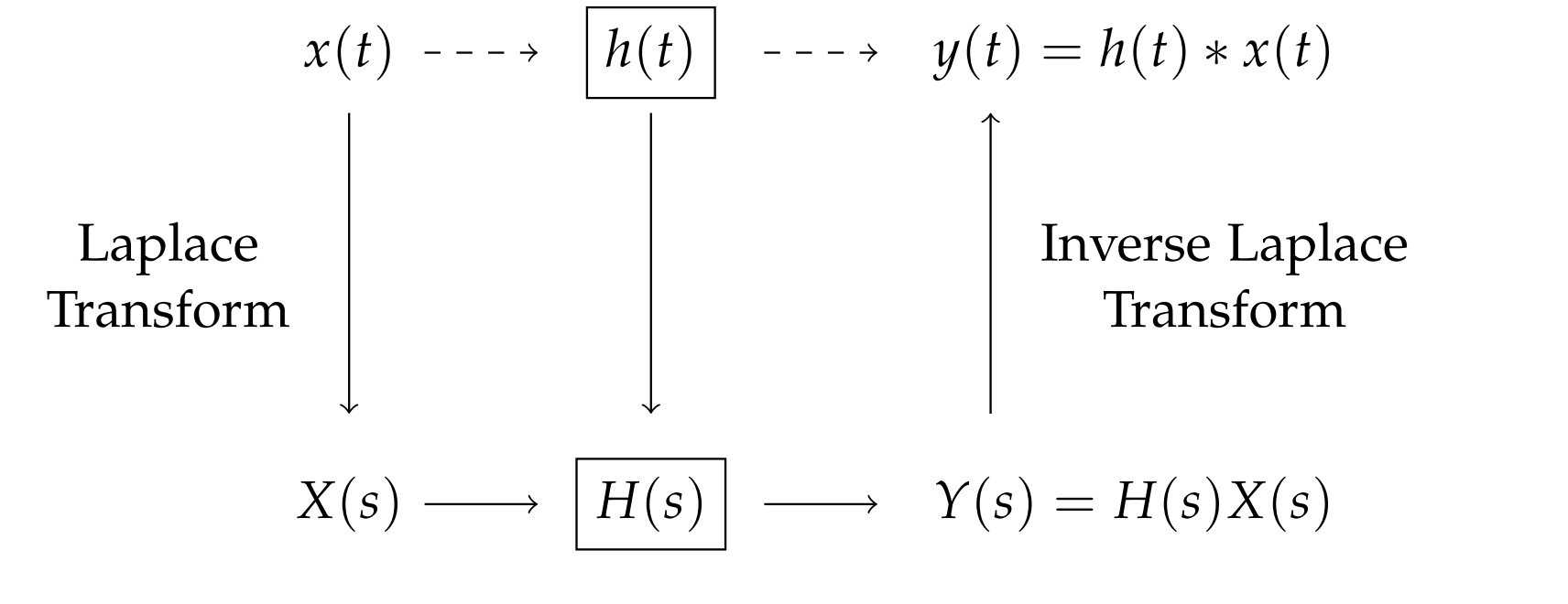
Laplace transforms also have proven useful in engineering for solving circuit problems and doing systems analysis. In Figure \(5.1\) it is shown that a signal \(x(t)\) is provided as input to a linear system, indicated by \(h(t)\). One is interested in the system output, \(y(t)\), which is given by a convolution of the input and system functions. By considering the transforms of \(x(t)\) and \(h(t)\), the transform of the output is given as a product of the Laplace transforms in the s-domain. In order to obtain the output, one needs to compute a convolution product for Laplace transforms similar to the convolution operation we had seen for Fourier transforms earlier in the chapter. Of course, for us to do this in practice, we have to know how to compute Laplace transforms.

Figure \(\PageIndex{1}\): A schematic depicting the use of Laplace transforms in systems theory.