5.6: Systems of ODEs

LAPACE TRANSFORMS ARE ALSO USEFUL for solving systems of differential equations. We will study linear systems of differential equation in Chapter 6. For now, we will just look at simple examples of the application of Laplace transforms.

An example of a system of two differential equations for two unknown functions, \(x(t)\) and \(y(t)\), is given by the pair of coupled differential equations

\[ \begin{aligned}&x^{\prime}=3 x+4 y \\ &y^{\prime}=2 x+y \end{aligned} \label{5.39} \]

Neither equation can be solved on its own without knowledge of the other unknown function. This is why they are called couple. We will also need initial values for the system. We will choose \(x(0)=1\) and \(y(0)=0\).

Now, what would happen if we were to take the Laplace transform of each equation? We can apply the rules as before. Letting the Laplace transforms of \(x(t)\) and \(y(t)\) be \(X(t)\) and \(Y(t)\), respectively, we have

\[ \begin{aligned}s X-1 &=3 X+4 Y, \\ s Y &=2 X+Y . \end{aligned} \label{5.40} \]

We have obtained a system of algebraic equations for \(X\) and \(Y\). Using standard methods, like Cramer’s Method, we can solve this system of two equations and two unknowns. First, we rewrite the equations as

\[ \begin{aligned}(s-3) X-4 Y &=1 \\ -2 X+(s-1) Y &=0 \end{aligned} \label{5.41} \]

Using Cramer’s (determinant) Rule for solving such systems, we have

\[X=\dfrac{\left|\begin{array}{cc} 1 & -4 \\ 0 & s-1 \end{array}\right|}{\left|\begin{array}{cc} s-3 & -4 \\ -2 & s-1 \end{array}\right|}, \quad Y=\dfrac{\left|\begin{array}{cc} s-3 & 1 \\ -2 & 0 \end{array}\right|}{\left|\begin{array}{cc} s-3 & -4 \\ -2 & s-1 \end{array}\right|} \nonumber \]

Note that the denominator in each solution is a \(2 \times 2\) determinant consisting of the coefficients of \(X\) and \(Y\) in the appropriate order. The numerators are the same determinant but with the right-hand side of the equation replacing the respective columns.

Computing the determinants, using

\[\left|\begin{array}{ll} a & b \\ c & d \end{array}\right|=a d-b c \nonumber \]

we have

\[X=\dfrac{1}{(s-3)(s-1)-8}, \quad Y=\dfrac{2}{(s-3)(s-1)-8} \nonumber \]

or

\[X=\dfrac{s-1}{s^{2}-4 s-5}, \quad Y=\dfrac{2}{s^{2}-4 s-5}\nonumber \]

We now know the Laplace transforms of the solutions, so a simple inverse Laplace transform is in order. The denominators are the same,

\[s^{2}-4 s-5=(s-5)(s+1)\nonumber \]

We can apply a partial fraction decomposition to each function to obtain

\[\begin{aligned}X &=\dfrac{s-1}{(s-5)(s+1)} \\ &=\dfrac{s-5+4}{(s-5)(s+1)} \\ &=\dfrac{1}{s+1}+\dfrac{4}{(s-5)(s+1)} \\ &=\dfrac{1}{s+1}+\dfrac{2}{3}\left[\dfrac{1}{s-5}-\dfrac{1}{s+1}\right] \\ &=\dfrac{2}{3} \dfrac{1}{s-5}+\dfrac{1}{3} \dfrac{1}{s+1} \\ Y &=\dfrac{2}{(s-5)(s+1)} \\ &=\dfrac{1}{3}\left[\dfrac{1}{s-5}-\dfrac{1}{s+1}\right] \end{aligned} \nonumber \]

So, the solutions to the system of differential equations is given by

\[ \begin{aligned}&x(t)=\dfrac{2}{3} e^{5} t+\dfrac{1}{3} e^{-t} \\ &y(t)=\dfrac{1}{3}\left(e^{5 t}-e^{-t}\right) \end{aligned} \nonumber \]

We can verify that \(x(0)=1\) and \(y(0)=0\).

\[ \begin{aligned}x^{\prime} &=\dfrac{10}{3} e^{5 t}-\dfrac{1}{3} e^{-t} \\ 3 x+4 y &=\left(2 e^{5 t}+e^{-t}\right)+\dfrac{4}{3}\left(e^{5 t}-e^{-t}\right) \\ &=\dfrac{10}{3} e^{5 t}-\dfrac{1}{3} e^{-t} \\ y^{\prime} &=\dfrac{5}{3} e^{5 t}+\dfrac{1}{3} e^{-t} \\ 2 x+y &=\left(\dfrac{4}{3} e^{5 t}+\dfrac{2}{3} e^{-t}\right)+\dfrac{1}{3}\left(e^{5 t}-e^{-t}\right) \\ &=\dfrac{5}{3} e^{5 t}+\dfrac{1}{3} e^{-t} \end{aligned} \label{5.43} \]

Example \(\PageIndex{1}\)

Determine the current in Figure \(\PageIndex{1}\) for the following values: \(i_1(0) = i_2(0) = i_3(0) = 0\) and

\[v(t)=\left\{\begin{array}{cl} v_{0}, & 0 \leq t \leq 3.0 \\ 0, & \text { otherwise } \end{array}\right. \nonumber \]

The problem can be modeled by a system of differential equations. In Figure \(\PageIndex{1}\) there are three currents indicated. Kirchoff’s Point(Junction) Rule indicates that \(i_{1}=i_{2}+i_{3}\).

Figure \(\PageIndex{1}\): A circuit with two loops containing two resistors and two inductors in parallel.

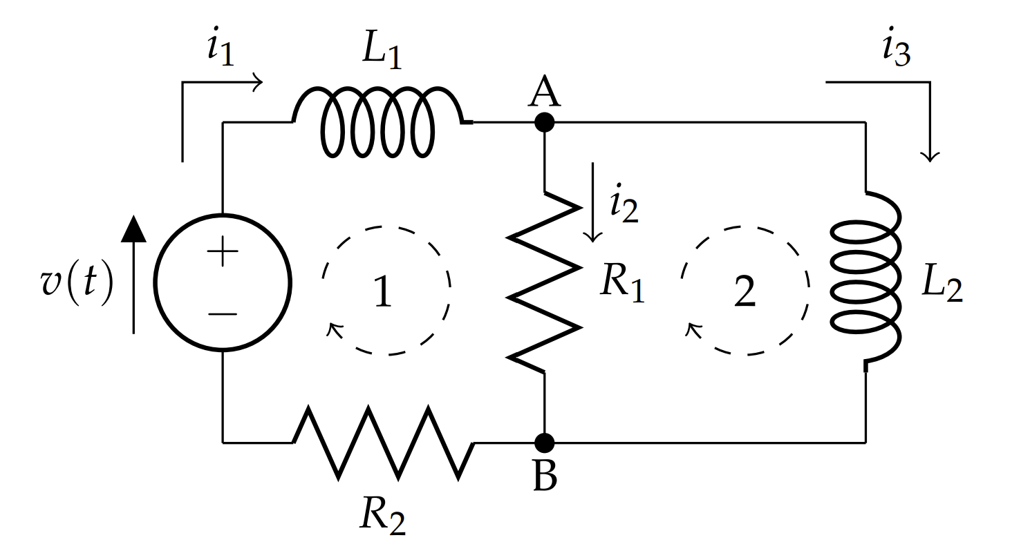
In order to apply Kirchoff’s Loop Rule, we need totally the potential drops and rises. For resistors, these come from Ohm’s Law, \(v=i R\), and for inductors, this comes from Faraday’s Law, \(v=L \dfrac{d i}{d t} .\) For the left loop (2), we have

\[L_{2} i_{3}^{\prime}=R_{1} i_{2} \nonumber \]

where the prime denotes the time derivative. For the right loop (1), we have

\[L_{1} i_{1}^{\prime}+R_{1} i_{2}+R_{2} i_{1}=v(t) \nonumber \]

We can use the Point Rule to eliminate one of the currents, \(i_{2}=i_{1}-i_{3}\), leaving the model as two first order differential equations,

\[ \begin{aligned}L_{2} i_{3}^{\prime}-R_{1}\left(i_{1}-i_{3}\right) &=0 \\ L_{1} i_{1}^{\prime}+R_{1}\left(i_{1}-i_{3}\right)+R_{2} i_{1} &=v(t) \end{aligned} \nonumber \]

Or

\[ \begin{aligned}L_{2} i_{3}^{\prime}-R_{1} i_{1}+R_{1} i_{3} &=0 \\ L_{1} i_{1}^{\prime}+\left(R_{1}+R_{2}\right) i_{1}-R_{1} i_{3} &=v_{0}(1-H(t-3)) \end{aligned} \nonumber \]

where \(H(t)\) is the Heaviside function.

Taking the Laplace transform, assuming that \(i_{1}(0)=i_{2}(0)=0\), we obtain the algebraic system of equations

\[ \begin{aligned}-R_{1} I_{1}+\left(s L_{2}+R_{1}\right) I_{3} &=0 \\ \left(s L_{1}+R_{1}+R_{2}\right) I_{1}-R_{1} I_{3} &=\dfrac{v_{0}}{s}\left(1-e^{-3 s}\right) \end{aligned} \nonumber \]

Here \(I_{1}(s)\) and \(I_{3}(s)\) are the Laplace transforms of \(i_{1}(t)\) and \(i_{3}(t)\), respectively.

As before, we use Cramer’s Rule to find the solutions.

\[\begin{aligned}
&I_{1}=\dfrac{\left|\begin{array}{cc}
0 & s L_{2}+R_{1} \\
\dfrac{v_{0}}{s}\left(1-e^{-3 s}\right) & -R_{1}
\end{array}\right|}{\left|\begin{array}{cc}
-R_{1} & s L_{2}+R_{1} \\
s L_{1}+R_{1}+R_{2} & -R_{1}
\end{array}\right|}\\
&=\dfrac{-v_{0}\left(s L_{2}+R_{1}\right)\left(1-e^{-3 s}\right)}{s\left[R_{1}^{2}-\left(s L_{2}+R_{1}\right)\left(s L_{1}+R_{1}+R_{2}\right)\right]}\\
&=\dfrac{v_{0}\left(s L_{2}+R_{1}\right)\left(1-e^{-3 s}\right)}{s\left[\left(L_{1} L_{2}\right) s^{2}+\left(R_{1} L_{1}+L_{2}\left(R_{1}+R_{2}\right)\right) s+R_{1} R_{2}\right]} .\\
&I_{3}=\dfrac{\left|\begin{array}{cc}
-R_{1} & 0 \\
s L_{1}+R_{1}+R_{2} & \dfrac{v_{0}}{s}\left(1-e^{-3 s}\right)
\end{array}\right|}{\left|\begin{array}{cc}
-R_{1} & s L_{2}+R_{1} \\
s L_{1}+R_{1}+R_{2} & -R_{1}
\end{array}\right|}\\
&=\dfrac{v_{0} R_{1}\left(1-e^{-3 s}\right)}{s\left[R_{1}^{2}-\left(s L_{2}+R_{1}\right)\left(s L_{1}+R_{1}+R_{2}\right)\right]}\\
&=\dfrac{-v_{0} R_{1}\left(1-e^{-3 s}\right)}{s\left[\left(L_{1} L_{2}\right) s^{2}+\left(R_{1} L_{1}+L_{2}\left(R_{1}+R_{2}\right)\right) s+R_{1} R_{2}\right]} .
\end{aligned}\label{5.44} \]

The denominator in these expressions cannot be factored. So, to make any further progress, one needs specific values for the constants. Let \(R_{1}=2.00 \Omega, R_{2}=18.0 \Omega, L_{1}=48.0 \mathrm{H}, L_{2}=6.00 \mathrm{H}\). and \(v_{0}=18\) V. Then,

\[ \begin{aligned}&I_{1}=\dfrac{3 s+1}{s(2 s+1)(4 s+1)}\left(1-e^{-3 s}\right) \\ &I_{3}=-\dfrac{1}{s(2 s+1)(4 s+1)}\left(1-e^{-3 s}\right) \end{aligned} \nonumber \]

Using partial fractions on the coefficient of \(\left(1-e^{-3 s}\right)\), we find that

\[ \begin{aligned}&\dfrac{3 s+1}{s(2 s+1)(4 s+1)}=\dfrac{1}{s}-\dfrac{2}{4 s+1}-\dfrac{1}{2 s+1} \\ &\dfrac{1}{s(2 s+1)(4 s+1)}=\dfrac{1}{s}-\dfrac{8}{4 s+1}+\dfrac{2}{2 s+1} \end{aligned} \nonumber \]

This gives

\[ \begin{aligned}&I_{1}=\left(\dfrac{1}{s}-\dfrac{1}{2} \dfrac{1}{s+\dfrac{1}{4}}-\dfrac{1}{2} \dfrac{1}{s+\dfrac{1}{2}}\right)\left(1-e^{-3 s}\right) \\ &I_{3}=\left(-\dfrac{1}{s}+\dfrac{2}{s+\dfrac{1}{4}}-\dfrac{1}{s+\dfrac{1}{2}}\right)\left(1-e^{-3 s}\right) \end{aligned} \nonumber \]

Taking the inverse Laplace transform, we find the solutions

\[i_{1}=1-\dfrac{1}{2} e^{-\dfrac{t}{4}}-\dfrac{1}{2} e^{-\dfrac{t}{2}}+\left(-1+\dfrac{1}{2} e^{-\dfrac{t-3}{4}}+\dfrac{1}{2} e^{-\dfrac{t-3}{2}}\right) H(t-3) \nonumber \]

\[=\left\{\begin{array}{cc}
1-\dfrac{1}{2} e^{-\dfrac{t}{4}}-\dfrac{1}{2} e^{-\dfrac{t}{2}}, & t \leq 3, \\
-\dfrac{1}{2}\left(1-e^{\dfrac{3}{4}}\right) e^{-\dfrac{t}{4}}-\dfrac{1}{2}\left(1-e^{\dfrac{3}{2}}\right) e^{-\dfrac{t}{2}}, & t \geq 3 .
\end{array}\right. \nonumber \]

Figure \(\PageIndex{2}\): A plot of the currents vs time for Example \(\PageIndex{1}\) with the voltage \(v(t)=v_{0}(1-H(t-3))\). The taller curve represents \(i_{1}\) and the other curve is \(-i_{3}\).

\[\begin{aligned}
i_{3} &=-1+2 e^{-\dfrac{t}{4}}-e^{-\dfrac{t}{2}}+\left(1-2 e^{-\dfrac{t-3}{4}}+e^{-\dfrac{t-3}{2}}\right) H(t-3) . \\
&=\left\{\begin{array}{cc}
-1+2 e^{-\dfrac{t}{4}}-e^{-\dfrac{t}{2}}, & t \leq 3 \\
2\left(1-e^{\dfrac{3}{4}}\right) e^{-\dfrac{t}{4}}-\left(1-e^{\dfrac{3}{2}}\right) e^{-\dfrac{t}{2}}, & t \geq 3
\end{array}\right.
\end{aligned} \nonumber \]

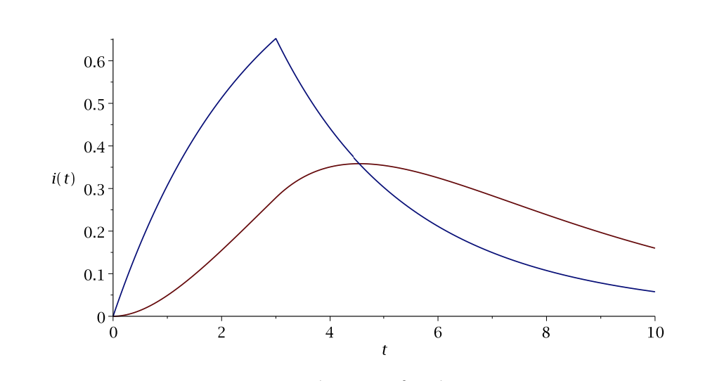
In Figure \(\PageIndex{2}\), we plot the currnts \(i_{1}\) and the other curve is \(-i\) is negative, indicating a flow in reverse of the direction in Figure \(\PageIndex{1}\). Not the sudden change in \(i[1]\) at \(t=3\), the time that the voltage is turned on.

One can easily change the time that the voltage is applied. Namely, if

\[v(t)=\left\{\begin{array}{cc}
v_{0}, & 0 \leq t \leq t_{0} \\
0, & \text { otherwise }
\end{array}\right. \nonumber \]

then the solutions are given by

\[ \begin{aligned}&i_{1}=1-\dfrac{1}{2} e^{-\dfrac{t}{4}}-\dfrac{1}{2} e^{-\dfrac{t}{2}}+\left(-1+\dfrac{1}{2} e^{-\dfrac{t-t_{0}}{4}}+\dfrac{1}{2} e^{-\dfrac{t-t_{0}}{2}}\right) H\left(t-t_{0}\right) \\ &i_{3}=-1+2 e^{-\dfrac{t}{4}}-e^{-\dfrac{t}{2}}+\left(1-2 e^{-\dfrac{t-t_{0}}{4}}+e^{-\dfrac{t-t_{0}}{2}}\right) H\left(t-t_{0}\right) \end{aligned} \nonumber \]

Figure \(\PageIndex{3}\): A plot of the currents vs time for Example \(\PageIndex{1}\) for the voltage given by \(v(t)=v_{0}(1-H(t-10))\). The taller curve represents \(i_{1}\) and the other curve is \(-i_3\)

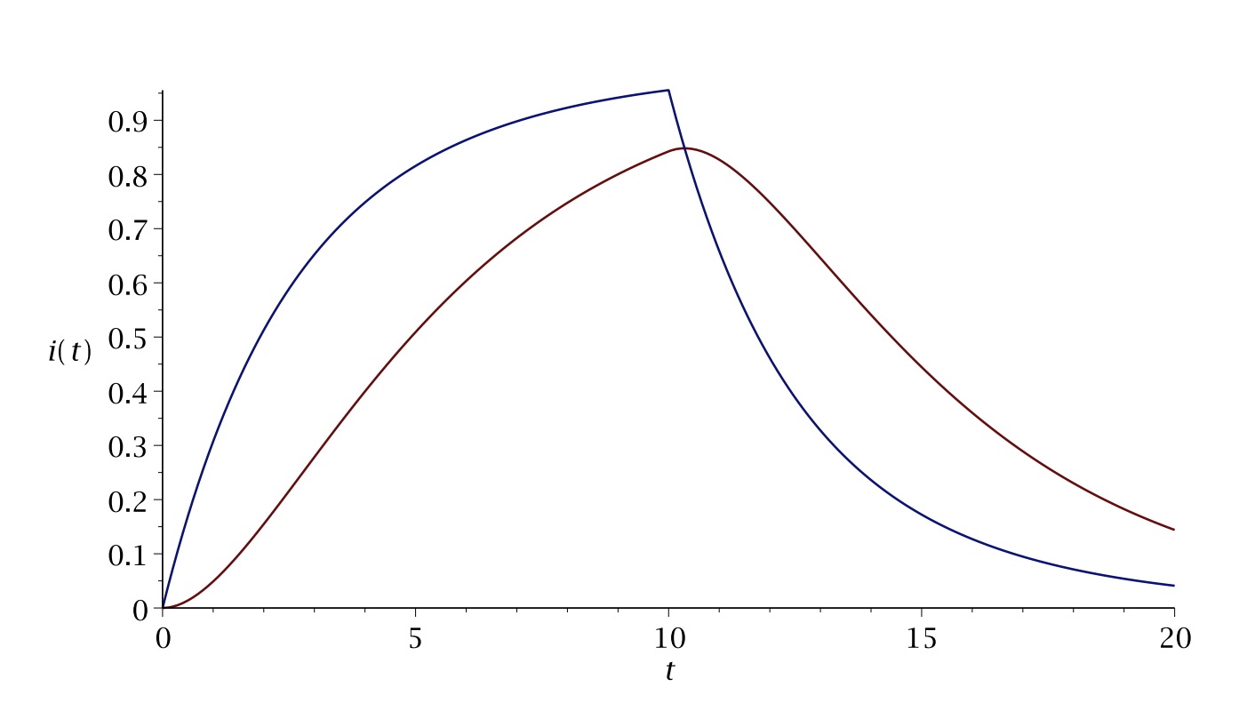
A plot of the currents for \(t_{0}=10\) are shown in Figure \(\PageIndex{3}\).