
6.1: Linear Systems
- Page ID
- 91123

6.1.1: Coupled Oscillators
IN SECTION \(3.5\) WE SAW THAT the numerical solution of second order equations, or higher, can be cast into systems of first order equations. Such systems are typically coupled in the sense that the solution of at least one of the equations in the system depends on knowing one of the other solutions in the system. In many physical systems this coupling takes place naturally. We will introduce a simple model in this section to illustrate the coupling of simple oscillators.
There are many problems in physics that result in systems of equations. This is because the most basic law of physics is given by Newton’s Second Law, which states that if a body experiences a net force, it will accelerate. Thus,
\[\sum \mathbf{F}=m \mathbf{a}\nonumber \]
Since \(\mathbf{a}=\ddot{\mathbf{x}}\) we have a system of second order differential equations in general for three dimensional problems, or one second order differential equation for one dimensional problems for a single mass.
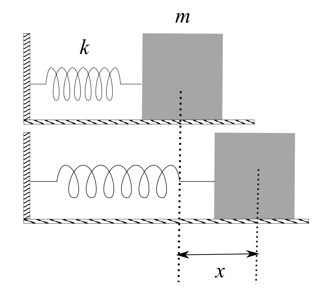
We have already seen the simple problem of a mass on a spring as shown in Figure 2.1. Recall that the net force in this case is the restoring force of the spring given by Hooke’s Law,
\[F_{S}=-k x \nonumber \]
where \(k>0\) is the spring constant and \(x\) is the elongation of the spring. When the spring constant is positive, the spring force is negative and when the spring constant is negative the spring force is positive. The equation for simple harmonic motion for the mass-spring system was found to be given by
\[m \ddot{x}+k x=0\nonumber \]
This second order equation can be written as a system of two first order equations in terms of the unknown position and velocity. We first set \(y=\dot{x}\). Noting that \(\ddot{x}=\dot{y}\), we rewrite the second order equation in terms of \(x\) and \(\dot{y}\). Thus, we have
\[\begin{array}{r} \dot{x}=y \\ \dot{y}=-\dfrac{k}{m} x \end{array} \label{6.1} \]
One can look at more complicated spring-mass systems. Consider two blocks attached with two springs as in Figure \(\PageIndex{2}.\) In this case we apply Newton’s second law for each block. We will designate the elongations of each spring from equilibrium as \(x_{1}\) and \(x_{2} .\) These are shown in Figure \(\PageIndex{2}.\)
For mass \(m_{1}\), the forces acting on it are due to each spring. The first spring with spring constant \(k_{1}\) provides a force on \(m_{1}\) of \(-k_{1} x_{1}\). The second spring is stretched, or compressed, based upon the relative locations of the two masses. So, the second spring will exert a force on \(m_{1}\) of \(k_{2}\left(x_{2}-x_{1}\right)\).
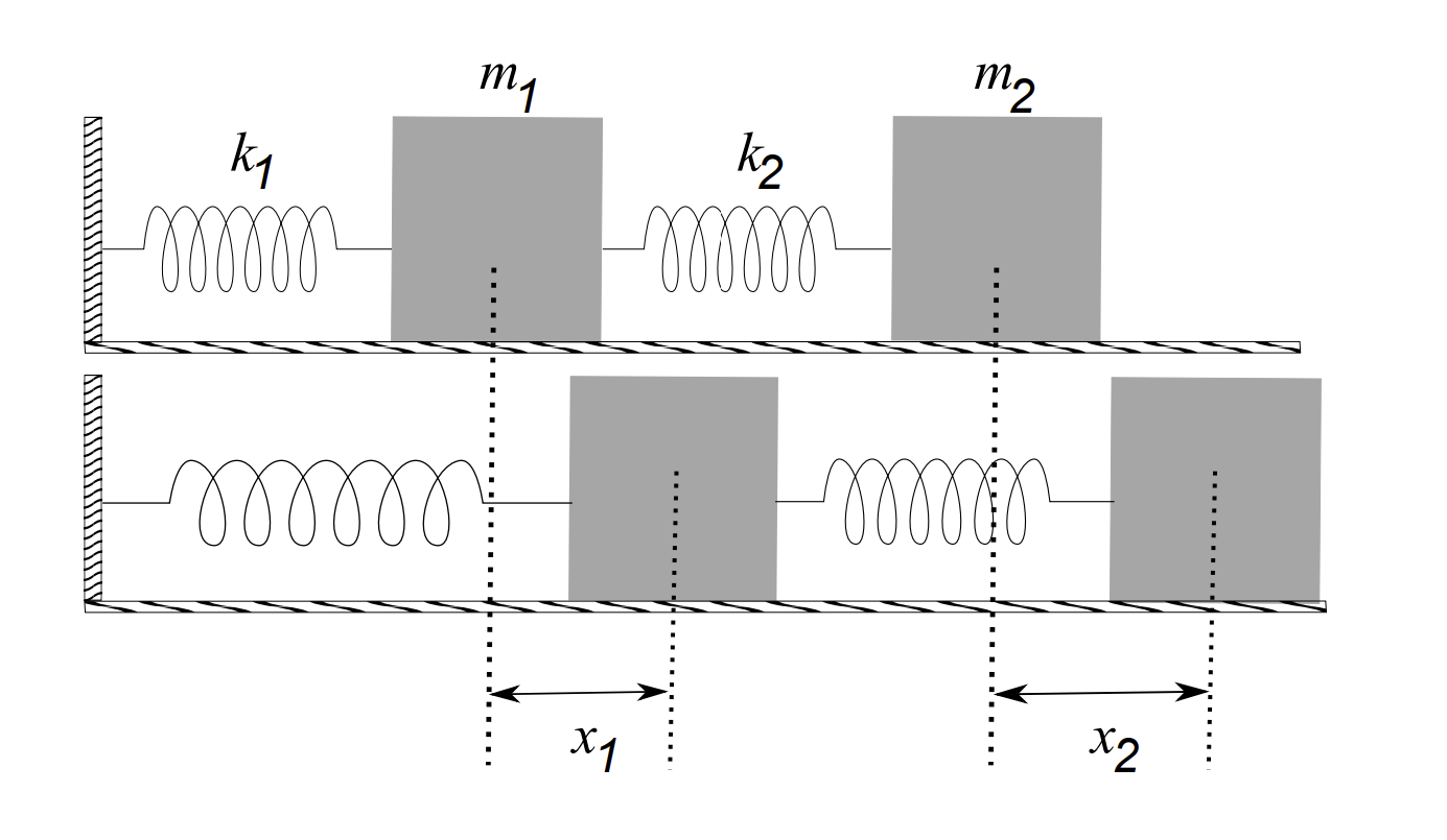
Similarly, the only force acting directly on mass \(m_{2}\) is provided by the restoring force from spring 2 . So, that force is given by \(-k_{2}\left(x_{2}-x_{1}\right)\). The reader should think about the signs in each case.
Putting this all together, we apply Newton’s Second Law to both masses. We obtain the two equations
\[ \begin{aligned} &m_{1} \ddot{x}_{1}=-k_{1} x_{1}+k_{2}\left(x_{2}-x_{1}\right) \\ &m_{2} \ddot{x}_{2}=-k_{2}\left(x_{2}-x_{1}\right) \end{aligned} \label{6.2} \]
Thus, we see that we have a coupled system of two second order differential equations. Each equation depends on the unknowns \(x_{1}\) and \(x_{2}\).
One can rewrite this system of two second order equations as a system of four first order equations by letting \(x_{3}=\dot{x}_{1}\) and \(x_{4}=\dot{x}_{2}\). This leads to the system
\[\dot{x}_{1}=x_{3}\nonumber \]
\[ \begin{aligned} \dot{x}_{2} &=x_{4} \\ \dot{x}_{3} &=-\dfrac{k_{1}}{m_{1}} x_{1}+\dfrac{k_{2}}{m_{1}}\left(x_{2}-x_{1}\right) \\ \dot{x}_{4} &=-\dfrac{k_{2}}{m_{2}}\left(x_{2}-x_{1}\right) \end{aligned} \label{6.3} \]
As we will see in the next chapter, this system can be written more compactly in matrix form:
\[\dfrac{d}{d t}\left(\begin{array}{c} x_{1} \\ x_{2} \\ x_{3} \\ x_{4} \end{array}\right)=\left(\begin{array}{cccc} 0 & 0 & 1 & 0 \\ 0 & 0 & 0 & 1 \\ -\dfrac{k_{1}+k_{2}}{m_{1}} & \dfrac{k_{2}}{m_{1}} & 0 & 0 \\ \dfrac{k_{2}}{m_{2}} & -\dfrac{k_{2}}{m_{2}} & 0 & 0 \end{array}\right)\left(\begin{array}{l} x_{1} \\ x_{2} \\ x_{3} \\ x_{4} \end{array}\right) \nonumber \]
We can solve this system of first order equations using matrix methods. However, we will first need to recall a few things from linear algebra. This will be done in the next chapter. For now, we will return to simpler systems and explore the behavior of typical solutions in planar systems.
6.1.2: Planar Systems
We NOW CONSIDER EXAMPLES of solving a coupled system of first order differential equations in the plane. We will focus on the theory of linear systems with constant coefficients. Understanding these simple systems will help in the study of nonlinear systems, which contain much more interesting behaviors, such as the onset of chaos. In the next chapter we will return to these systems and describe a matrix approach to obtaining the solutions.
A general form for first order systems in the plane is given by a system of two equations for unknowns \(x(t)\) and \(y(t)\) :
\[ \begin{aligned} &x^{\prime}(t)=P(x, y, t) \\ &y^{\prime}(t)=Q(x, y, t) \end{aligned} \label{6.5} \]
An autonomous system is one in which there is no explicit time dependence:
Autonomous systems.
\[ \begin{aligned} & x^{\prime}(t)=P(x, y) \\ & y^{\prime}(t)=Q(x, y) . \end{aligned} \label{6.6} \]
Otherwise the system is called nonautonomous.
A linear system takes the form
\[ \begin{aligned} &x^{\prime}=a(t) x+b(t) y+e(t) \\ &y^{\prime}=c(t) x+d(t) y+f(t) \end{aligned} \label{6.7} \]
A homogeneous linear system results when \(e(t)=0\) and \(f(t)=0 .\)
A linear, constant coefficient system of first order differential equations is given by
\[\begin{aligned} &x^{\prime}=a x+b y+e \\ &y^{\prime}=c x+d y+f \end{aligned} \label{6.8} \]
A linear, homogeneous system of constant coefficient first order differential equations in the plane.
We will focus on linear, homogeneous systems of constant coefficient first order differential equations:
\[ \begin{array}{|l} x^{\prime}=a x+b y \\ y^{\prime}=c x+d y. \end{array} \label{6.9} \]
As we will see later, such systems can result by a simple translation of the unknown functions. These equations are said to be coupled if either \(b \neq 0\) or \(c \neq 0\).
We begin by noting that the system Equation \(\PageIndex{9}\) can be rewritten as a second order constant coefficient linear differential equation, which we already know how to solve. We differentiate the first equation in system Equation \(\PageIndex{9}\) and systematically replace occurrences of \(y\) and \(y^{\prime}\), since we also know from the first equation that \(y=\dfrac{1}{b}\left(x^{\prime}-a x\right)\). Thus, we have
\[ \begin{aligned} x^{\prime \prime} &=a x^{\prime}+b y^{\prime} \\ &=a x^{\prime}+b(c x+d y) \\ &=a x^{\prime}+b c x+d\left(x^{\prime}-a x\right) \end{aligned} \label{6.10} \]
Rewriting the last line, we have
\[x^{\prime \prime}-(a+d) x^{\prime}+(a d-b c) x=0 \nonumber \]
This is a linear, homogeneous, constant coefficient ordinary differential equation. We know that we can solve this by first looking at the roots of the characteristic equation
\[r^{2}-(a+d) r+a d-b c=0 \nonumber \]
and writing down the appropriate general solution for \(x(t)\). Then we can find \(y(t)\) using
Equation \(\PageIndex{9}\):
\[y=\dfrac{1}{b}\left(x^{\prime}-a x\right)\nonumber \]
We now demonstrate this for a specific example.
Consider the system of differential equations
\[ \begin{aligned} &x^{\prime}=-x+6 y \\ &y^{\prime}=x-2 y \end{aligned} \label{6.13} \]
Carrying out the above outlined steps, we have that \(x^{\prime \prime}+3 x^{\prime}-4 x=0\). This can be shown as follows:
\[ \begin{aligned} x^{\prime \prime} &=-x^{\prime}+6 y^{\prime} \\ &=-x^{\prime}+6(x-2 y) \\ &=-x^{\prime}+6 x-12\left(\dfrac{x^{\prime}+x}{6}\right) \\ &=-3 x^{\prime}+4 x \end{aligned} \label{6.14} \]
The resulting differential equation has a characteristic equation of \(r^{2}+3 r-4=0\). The roots of this equation are \(r=1,-4\). Therefore, \(x(t)=c_{1} e^{t}+c_{2} e^{-4 t}\). But, we still need \(y(t)\). From the first equation of the system we have
\[y(t)=\dfrac{1}{6}\left(x^{\prime}+x\right)=\dfrac{1}{6}\left(2 c_{1} e^{t}-3 c_{2} e^{-4 t}\right) \nonumber \]
Thus, the solution to the system is
\[ \begin{aligned} &x(t)=c_{1} e^{t}+c_{2} e^{-4 t} \\ &y(t)=\dfrac{1}{3} c_{1} e^{t}-\dfrac{1}{2} c_{2} e^{-4 t} \end{aligned} \label{6.15} \]
Sometimes one needs initial conditions. For these systems we would specify conditions like \(x(0)=x_{0}\) and \(y(0)=y_{0}\). These would allow the determination of the arbitrary constants as before.
Solving systems with initial conditions.
Solve
\[ \begin{aligned} &x^{\prime}=-x+6 y \\ &y^{\prime}=x-2 y \end{aligned} \label{6.16} \]
given \(x(0)=2, y(0)=0\).
We already have the general solution of this system in Equation \(\PageIndex{15}\). Inserting the initial conditions, we have
\[ \begin{aligned} &2=c_{1}+c_{2} \\ &0=\dfrac{1}{3} c_{1}-\dfrac{1}{2} c_{2} \end{aligned} \label{6.17} \]
Solving for \(c_{1}\) and \(c_{2}\) gives \(c_{1}=6 / 5\) and \(c_{2}=4 / 5 .\) Therefore, the solution of the initial value problem is
\[ \begin{aligned} &x(t)=\dfrac{2}{5}\left(3 e^{t}+2 e^{-4 t}\right) \\ &y(t)=\dfrac{2}{5}\left(e^{t}-e^{-4 t}\right) \end{aligned}\label{6.18} \]
6.1.3: Equilibrium Solutions and Nearby Behaviors
IN STUDYING SYSTEMS OF DIFFERENTIAL EQUATIONS, it is often useful to study the behavior of solutions without obtaining an algebraic form for the solution. This is done by exploring equilibrium solutions and solutions nearby equilibrium solutions. Such techniques will be seen to be useful later in studying nonlinear systems.
We begin this section by studying equilibrium solutions of system Equation \(\PageIndex{8}\). For equilibrium solutions the system does not change in time. Therefore, equilibrium solutions satisfy the equations \(x^{\prime}=0\) and \(y^{\prime}=0\). Of course, this can only happen for constant solutions. Let \(x_{0}\) and \(y_{0}\) be the (constant) equilibrium solutions. Then, \(x_{0}\) and \(y_{0}\) must satisfy the system
Equilibrium solutions.
\[ \begin{aligned} 0 &=a x_{0}+b y_{0}+e \\ 0 &=c x_{0}+d y_{0}+f \end{aligned} \label{6.19} \]
This is a linear system of nonhomogeneous algebraic equations. One only has a unique solution when the determinant of the system is not zero, i.e., \(a d-b c \neq 0 .\) Using Cramer’s (determinant) Rule for solving such systems, we have
\[x_{0}=-\dfrac{\left|\begin{array}{ll}e & b \\ f & d\end{array}\right|}{\left|\begin{array}{ll}a & b \\ c & d\end{array}\right|}, \quad y_{0}=-\dfrac{\left|\begin{array}{ll}a & e \\ c & f\end{array}\right|}{\left|\begin{array}{ll}a & b \\ c & d\end{array}\right|} \nonumber \]
If the system is homogeneous, \(e=f=0\), then we have that the origin is the equilibrium solution; i.e., \(\left(x_{0}, y_{0}\right)=(0,0)\). Often we will have this case since one can always make a change of coordinates from \((x, y)\) to \((u, v)\) by \(u=x-x_{0}\) and \(v=y-y_{0} .\) Then, \(u_{0}=v_{0}=0 .\)
Next we are interested in the behavior of solutions near the equilibrium solutions. Later this behavior will be useful in analyzing more complicated nonlinear systems. We will look at some simple systems that are readily solved.
Consider the system
\[ \begin{gathered} x^{\prime}=-2 x \\ y^{\prime}=-y \end{gathered} \label{6.21} \]
This is a simple uncoupled system. Each equation is simply solved to give
\[x(t)=c_{1} e^{-2 t} \text { and } y(t)=c_{2} e^{-t} \nonumber \]
In this case we see that all solutions tend towards the equilibrium point, \((0,0)\). This will be called a stable node, or a sink.
Before looking at other types of solutions, we will explore the stable node in the above example. There are several methods of looking at the behavior of solutions. We can look at solution plots of the dependent versus the independent variables, or we can look in the \(x y\)-plane at the parametric curves \((x(t), y(t))\).
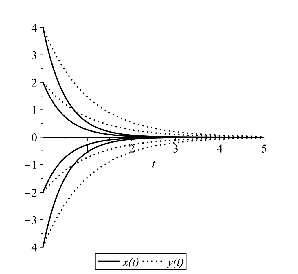
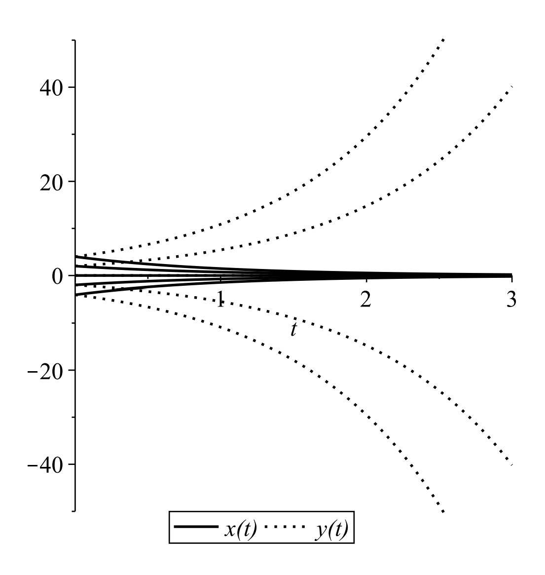
Solution Plots: One can plot each solution as a function of \(t\) given a set of initial conditions. Examples are shown in Figure \(\PageIndex{3}\) for several initial conditions. Note that the solutions decay for large \(t .\) Special cases result for various initial conditions. Note that for \(t=0, x(0)=c_{1}\) and \(y(0)=c_{2} .\) (Of course, one can provide initial conditions at any \(t=t_{0} .\) It is generally easier to pick \(t=0\) in our general explanations.) If we pick an initial condition with \(c_{1}=0\), then \(x(t)=0\) for all \(t\). One obtains similar results when setting \(y(0)=0\).
Phase Portrait: There are other types of plots which can provide additional information about the solutions even if we cannot find the exact solutions as we can for these simple examples. In particular, one can consider the solutions \(x(t)\) and \(y(t)\) as the coordinates along a parameterized path, or curve, in the plane: \(\mathbf{r}=(x(t), y(t))\) Such curves are called trajectories or orbits. The \(x y\)-plane is called the phase plane and a collection of such orbits gives a phase portrait for the family of solutions of the given system.
One method for determining the equations of the orbits in the phase plane is to eliminate the parameter \(t\) between the known solutions to get a relationship between \(x\) and \(y\). Since the solutions are known for the last example, we can do this, since the solutions are known. In particular, we have
\[x=c_{1} e^{-2 t}=c_{1}\left(\dfrac{y}{c_{2}}\right)^{2} \equiv A y^{2}. \nonumber \]
Another way to obtain information about the orbits comes from noting that the slopes of the orbits in the \(x y\)-plane are given by \(d y / d x\). For autonomous systems, we can write this slope just in terms of \(x\) and \(y\). This leads to a first order differential equation, which possibly could be solved analytically or numerically.
First we will obtain the orbits for Example \(\PageIndex{3}\) by solving the corresponding slope equation. Recall that for trajectories defined parametrically by \(x=x(t)\) and \(y=y(t)\), we have from the Chain Rule for \(y=y(x(t))\) that
\[\dfrac{d y}{d t}=\dfrac{d y}{d x} \dfrac{d x}{d t} \nonumber \]
Therefore,
The Slope of a parametric curve.
\[\dfrac{d y}{d x}=\dfrac{\dfrac{d y}{d t}}{\dfrac{d x}{d t}} \nonumber \]
For the system in Equation \(\PageIndex{21}\) we use Equation \(\PageIndex{22}\) to obtain the equation for the slope at a point on the orbit:
\[\dfrac{d y}{d x}=\dfrac{y}{2 x}\nonumber \]
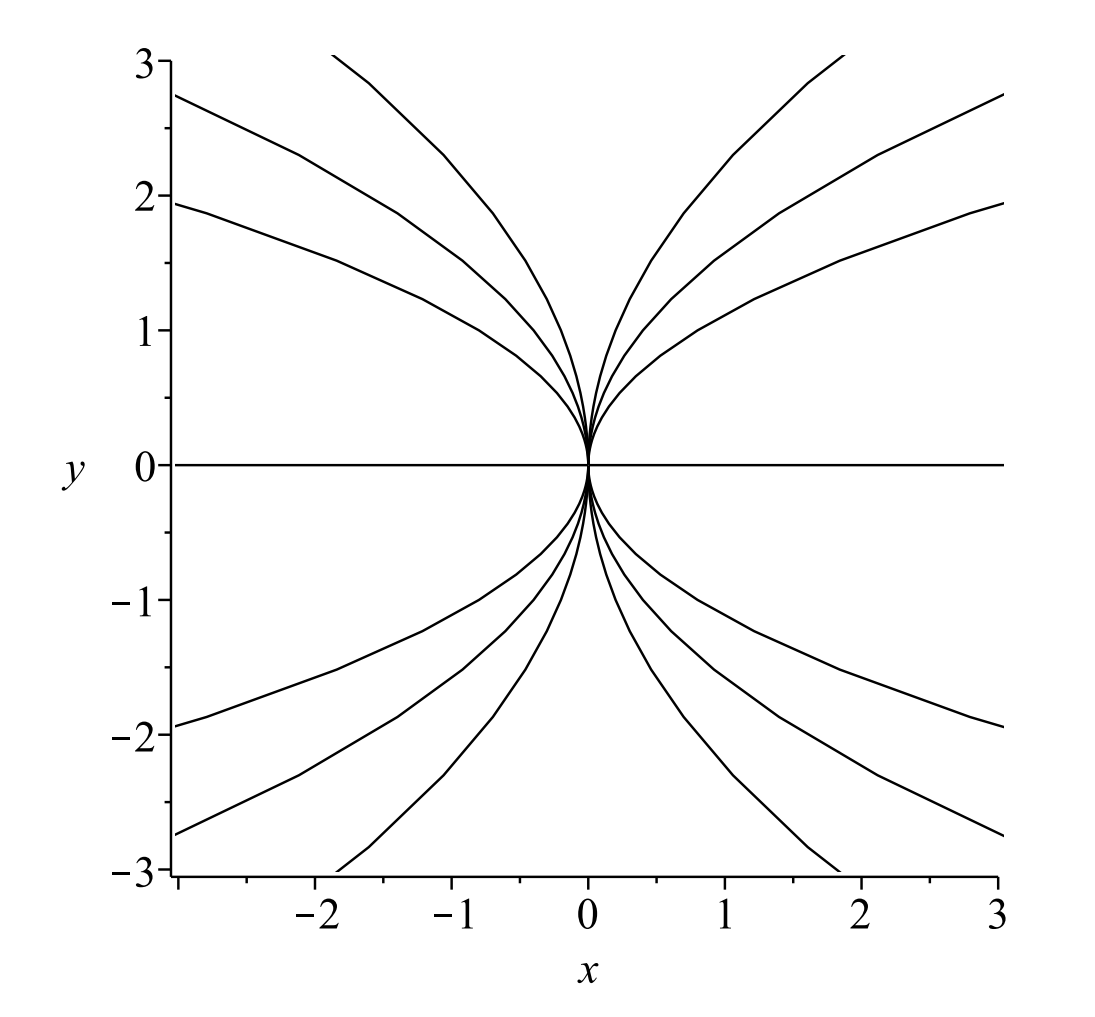
The general solution of this first order differential equation is found using
separation of variables as \(x=A y^{2}\) for \(A\) an arbitrary constant. Plots of these solutions in the phase plane are given in Figure \(\PageIndex{4}\). [Note that this is the same form for the orbits that we had obtained above by eliminating \(t\) from the solution of the system.]
Once one has solutions to differential equations, we often are interested in the long time behavior of the solutions. Given a particular initial condition \(\left(x_{0}, y_{0}\right)\), how does the solution behave as time increases? For orbits near an equilibrium solution, do the solutions tend towards, or away from, the equilibrium point? The answer is obvious when one has the exact solutions \(x(t)\) and \(y(t)\). However, this is not always the case.
Let’s consider the above example for initial conditions in the first quadrant of the phase plane. For a point in the first quadrant we have that
\[d x / d t=-2 x<0\nonumber \]
meaning that as \(t \rightarrow \infty, x(t)\) get more negative. Similarly,
\[d y / d t=-y<0 \nonumber \]
indicating that \(y(t)\) is also getting smaller for this problem. Thus, these orbits tend towards the origin as \(t \rightarrow \infty\). This qualitative information was obtained without relying on the known solutions to the problem.
Direction Fields: Another way to determine the behavior of the solutions of the system of differential equations is to draw the direction field. A direction field is a vector field in which one plots arrows in the direction of tangents to the orbits at selected points in the plane. This is done because the slopes of the tangent lines are given by \(d y / d x\). For the general system Equation \(\PageIndex{9}\), the slope is
\[\dfrac{d y}{d x}=\dfrac{c x+d y}{a x+b y}\nonumber \]
This is a first order differential equation which can be solved as we show in the following examples.
Draw the direction field for Example \(\PageIndex{3}\).
We can use software to draw direction fields. However, one can sketch these fields by hand. We have that the slope of the tangent at this point is given by
\[\dfrac{d y}{d x}=\dfrac{-y}{-2 x}=\dfrac{y}{2 x} \nonumber \]
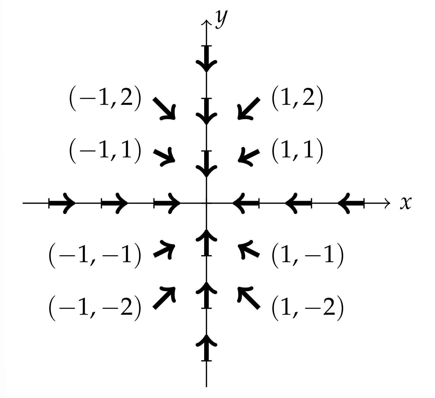
For each point in the plane one draws a piece of tangent line with this slope. In Figure \(\PageIndex{5}\) we show a few of these. For \((x, y)=(1,1)\) the slope is \(d y / d x=1 / 2 .\) So, we draw an arrow with slope \(1 / 2\) at this point. From system Equation \(\PageIndex{21}\), we have that \(x^{\prime}\) and \(y^{\prime}\) are both negative at this point. Therefore, the vector points down and to the left.
We can do this for several points, as shown in Figure \(\PageIndex{5}.\) Sometimes one can quickly sketch vectors with the same slope. For this example, when \(y=0\), the slope is zero and when \(x=0\) the slope is infinite. So, several vectors can be provided. Such vectors are tangent to curves known as isoclines in which \(\dfrac{d y}{d x}=\) constant.
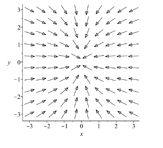
It is often difficult to provide an accurate sketch of a direction field. Computer software can be used to provide a better rendition. For Example \(\PageIndex{3}\) the direction field is shown in Figure \(\PageIndex{6}\). Looking at this direction field, one can begin to "see" the orbits by following the tangent vectors.
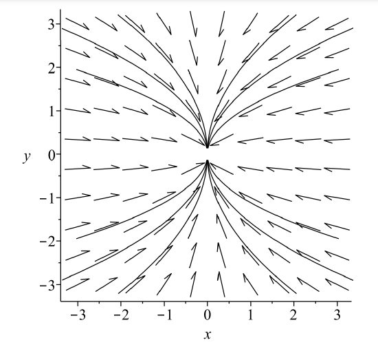
Of course, one can superimpose the orbits on the direction field. This is shown in Figure \(\PageIndex{7}\). Are these the patterns you saw in Figure \(\PageIndex{6}\)?
In this example we see all orbits "flow" towards the origin, or equilibrium point. Again, this is an example of what is called a stable node or a sink. (Imagine what happens to the water in a sink when the drain is unplugged.)
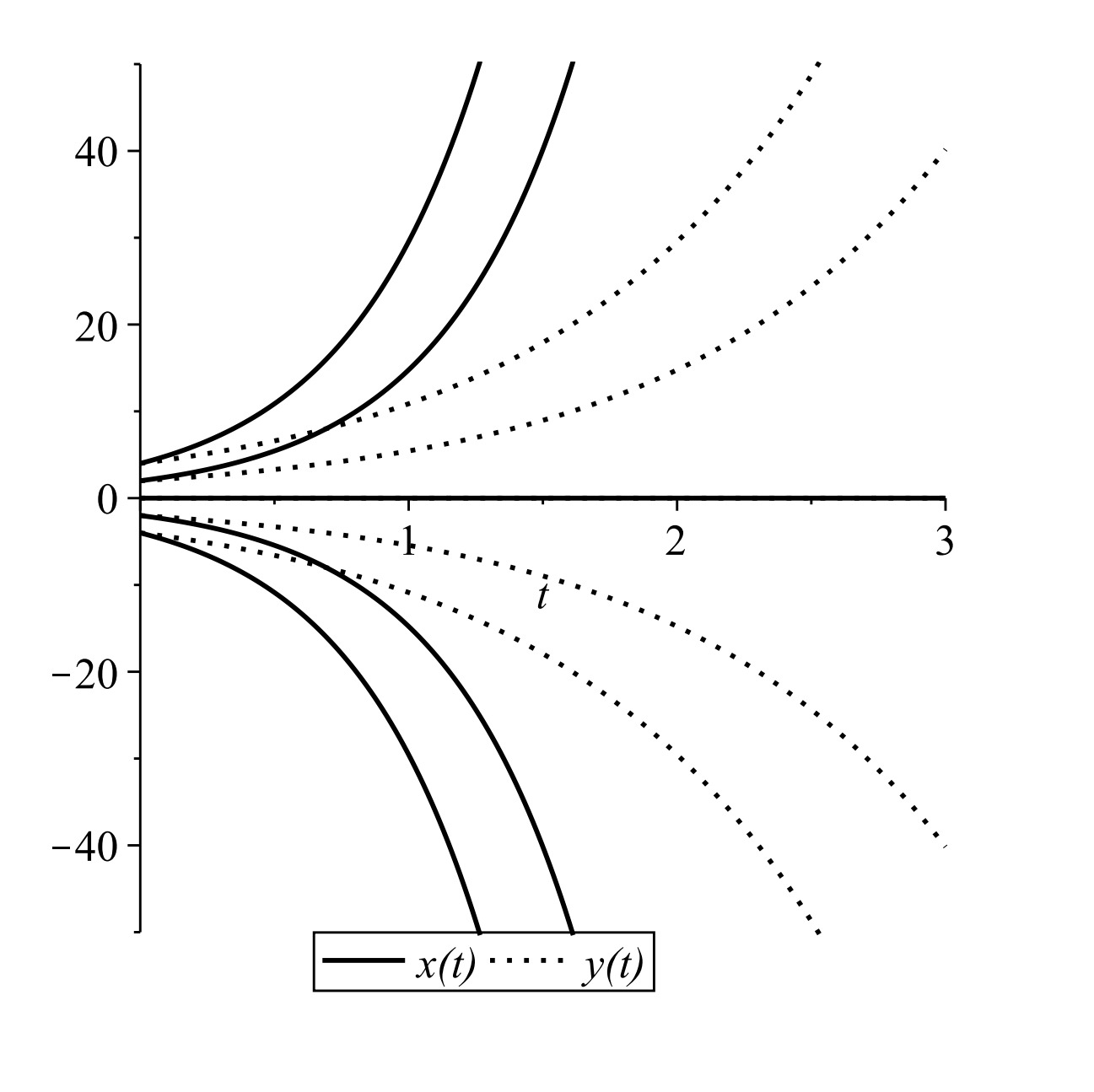
This is another uncoupled system. The solutions are again simply gotten by integration. We have that \(x(t)=c_{1} e^{-t}\) and \(y(t)=c_{2} e^{t} .\) Here we have that \(x\) decays as \(t\) gets large and \(y\) increases as \(t\) gets large. In particular, if one picks initial conditions with \(c_{2}=0\), then orbits follow the \(x\)-axis towards the origin. For initial points with \(c_{1}=0\), orbits originating on the \(y\)-axis will flow away from the origin. Of course, in these cases the origin is an equilibrium point and once at equilibrium, one remains there.
In fact, there is only one line on which to pick initial conditions such that the orbit leads towards the equilibrium point. No matter how small \(c_{2}\) is, sooner, or later, the exponential growth term will dominate the solution. One can see this behavior in Figure \(\PageIndex{8}\)\).
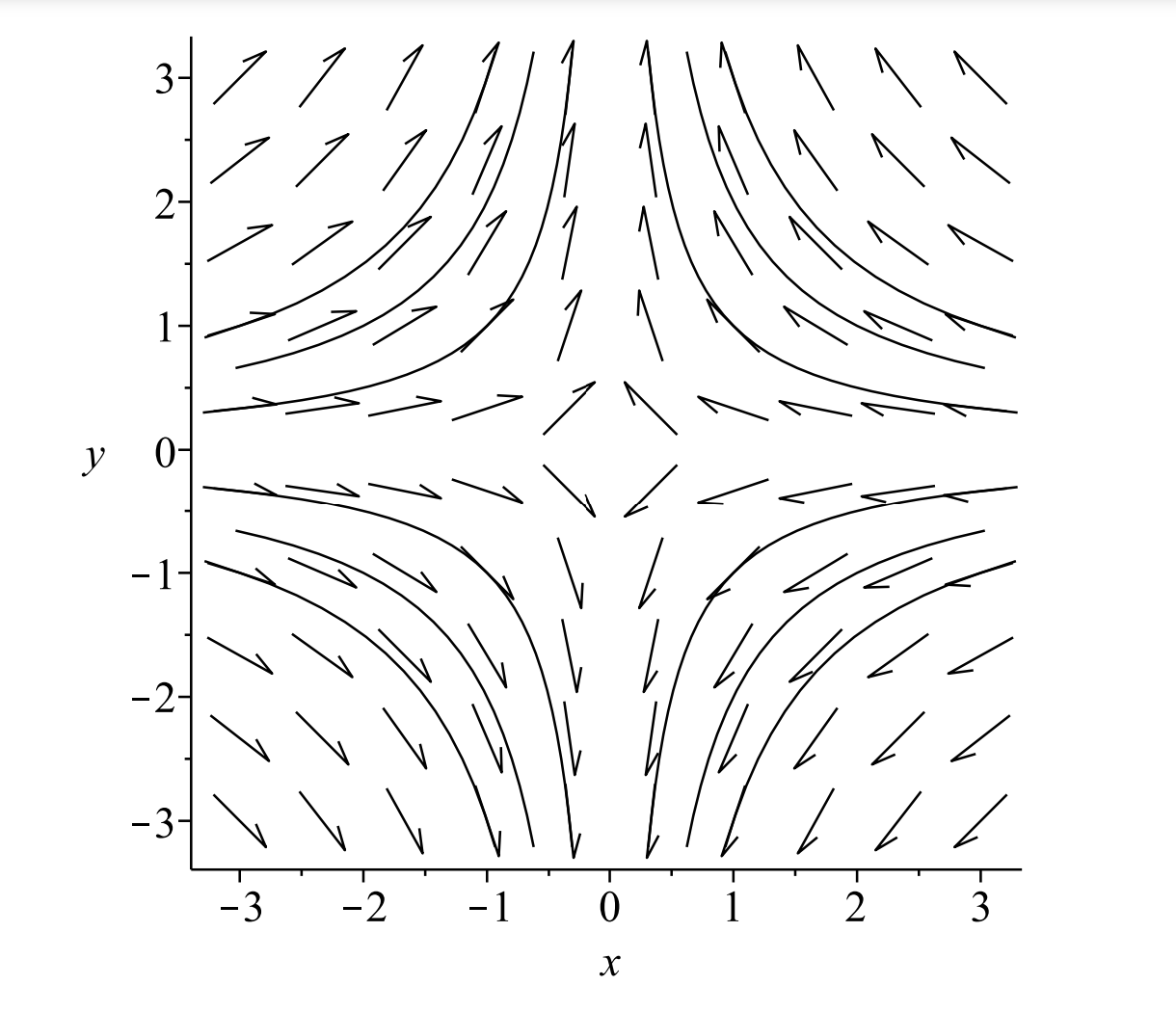
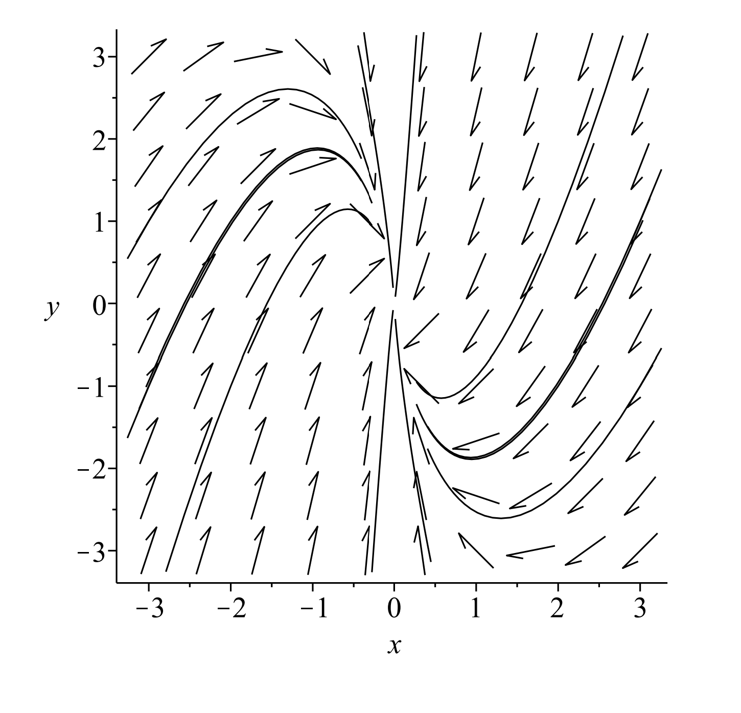
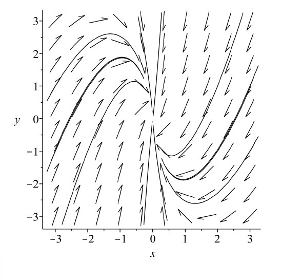
Consider the system
\[ \begin{aligned} &x^{\prime}=-x \\ &y^{\prime}=y. \end{aligned} \label{6.23} \]
Similar to the first example, we can look at plots of solutions orbits in the phase plane. These are given by Figures \(\PageIndex{8} - \PageIndex{9}.\) The orbits can be obtained from the system as
\[\dfrac{d y}{d x}=\dfrac{d y / d t}{d x / d t}=-\dfrac{y}{x} \nonumber \]
The solution is \(y=\dfrac{A}{x}\). For different values of \(A \neq 0\) we obtain a family of hyperbolae. These are the same curves one might obtain for the level curves of a surface known as a saddle surface, \(z=x y\). Thus, this type of equilibrium point is classified as a saddle point. From the phase portrait we can verify that there are many orbits that lead away from the origin (equilibrium point), but there is one line of initial conditions that leads to the origin and that is the \(x\)-axis. In this case, the line of initial conditions is given by the \(x\)-axis.
\[\begin{aligned} &x^{\prime}=2 x \\ &y^{\prime}=y. \end{aligned} \label{6.24} \]
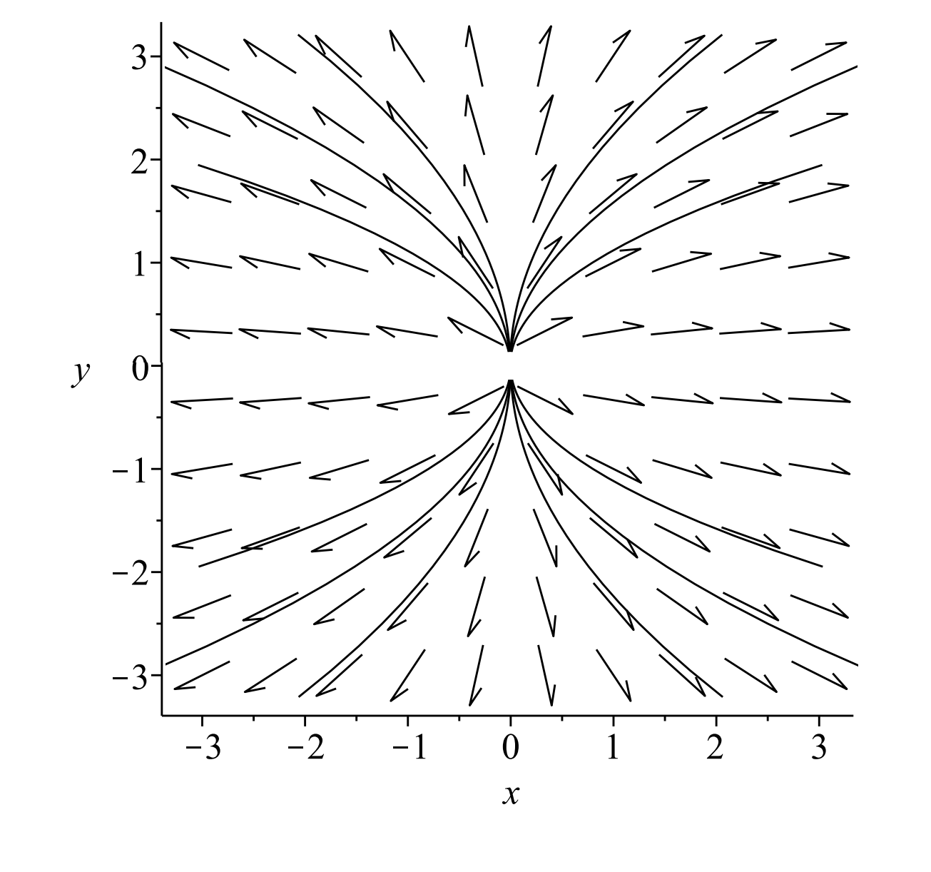
This example is similar to Example \(\PageIndex{3}\). The solutions are obtained by replacing \(t\) with \(-t\). The solutions, orbits, and direction fields can be seen in Figures \(\PageIndex{10} - \PageIndex{11}\). This is once again a node, but all orbits lead away from the equilibrium point. It is called an unstable node or a source.
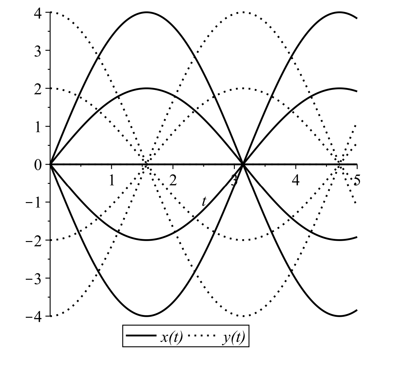
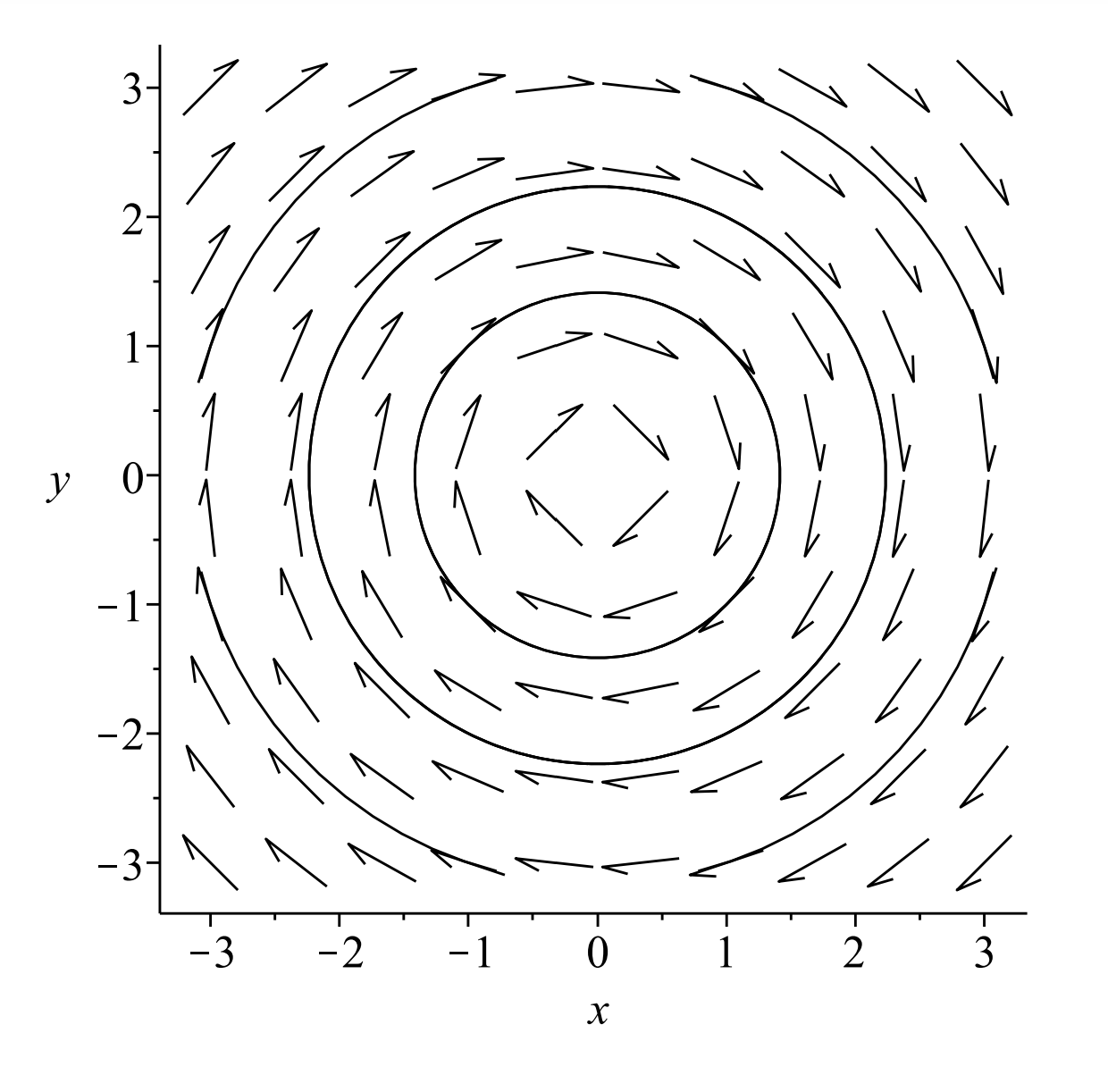
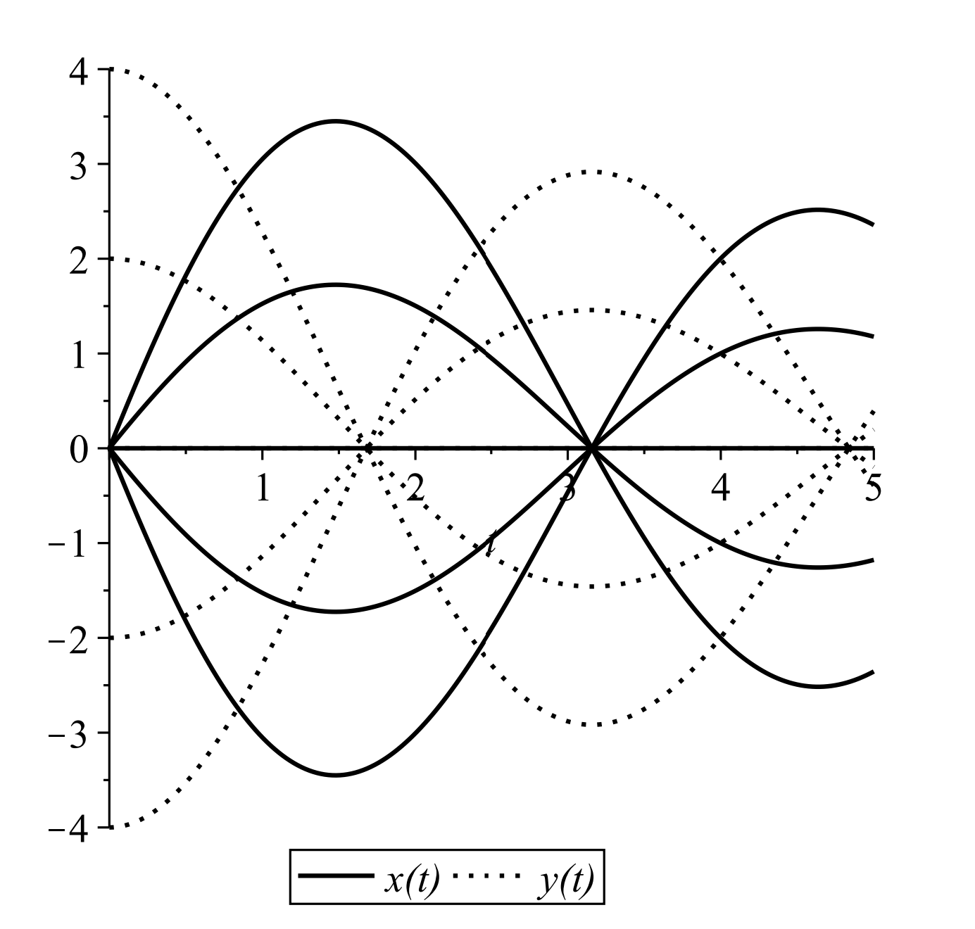
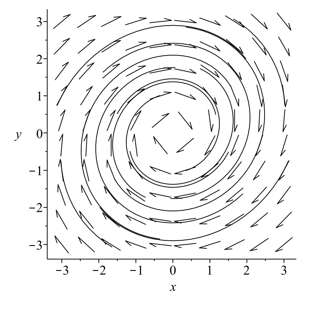
\[ \begin{aligned} &x^{\prime}=y \\ &y^{\prime}=-x \end{aligned} \label{6.25} \]
This system is a simple, coupled system. Neither equation can be solved without some information about the other unknown function. However, we can differentiate the first equation and use the second equation to obtain
\[x^{\prime \prime}+x=0\nonumber \]
We recognize this equation as one that appears in the study of simple harmonic motion. The solutions are pure sinusoidal oscillations:
\[x(t)=c_{1} \cos t+c_{2} \sin t, \quad y(t)=-c_{1} \sin t+c_{2} \cos t \nonumber \]
In the phase plane the trajectories can be determined either by looking at the direction field, or solving the first order equation
\[\dfrac{dy}{dx}=-\dfrac{x}{y} \nonumber \]
Performing a separation of variables and integrating, we find that
\[x^{2}+y^{2}=C\nonumber \]
Thus, we have a family of circles for \(C>0\). (Can you prove this using the general solution?) Looking at the results graphically in Figures \(\PageIndex{12} -\PageIndex{13}\) confirms this result. This type of point is called a center.
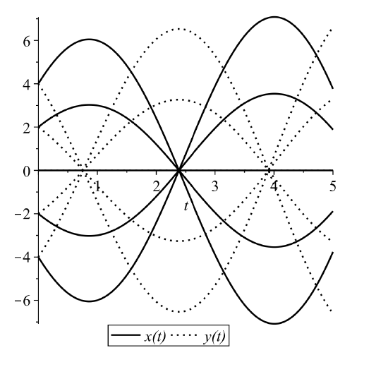
\[ \begin{aligned} x' &=\alpha x+y \\ y' &=-x \end{aligned} \label{6.26} \]
In this example, we will see an additional set of behaviors of equilibrium points in planar systems. We have added one term, \(\alpha x\), to the system in Example \(\PageIndex{7}\). We will consider the effects for two specific values of the parameter: \(\alpha=0.1,-0.2\). The resulting behaviors are shown in the Figures 6.15-6.18. We see orbits that look like spirals. These orbits are stable and unstable spirals (or foci, the plural of focus.)
We can understand these behaviors by once again relating the system of first order differential equations to a second order differential equation. Using the usual method for obtaining a second order equation form a system, we find that \(x(t)\) satisfies the differential equation
\[x''-\alpha x' + x =0 \nonumber \]
We recall from our first course that this is a form of damped simple harmonic motion. The characteristic equation is \(r^{2}-\alpha r+1=0 .\) The solution of this quadratic equation is
\[r=\dfrac{\alpha \pm \sqrt{\alpha^{2}-4}}{2} \nonumber \]
There are five special cases to consider as shown in the below classification.
Classification of Solutions of \(x^{\prime \prime}-\alpha x^{\prime}+x=0\)
- \(\alpha=-2\). There is one real solution. This case is called critical damping since the solution \(r=-1\) leads to exponential decay. The solution is \(x(t)=\left(c_{1}+c_{2} t\right) e^{-t} .\)
- \(\alpha<-2\). There are two real, negative solutions, \(r=-\mu,-v, \mu, v>0\). The solution is \(x(t)=c_{1} e^{-\mu t}+c_{2} e^{-v t}\). In this case we have what is called overdamped motion. There are no oscillations
- \(-2<\alpha<0 .\) There are two complex conjugate solutions \(r=\alpha / 2 \pm i \beta\) with real part less than zero and \(\beta=\dfrac{\sqrt{4-\alpha^{2}}}{2}\). The solution is \(x(t)=\) \(\left(c_{1} \cos \beta t+c_{2} \sin \beta t\right) e^{\alpha t / 2} .\) Since \(\alpha<0\), this consists of a decaying exponential times oscillations. This is often called an underdamped oscillation.
- \(\alpha=0\). This leads to simple harmonic motion.
- \(0<\alpha<2\). This is similar to the underdamped case, except \(\alpha>0\). The solutions are growing oscillations.
- \(\alpha=2 .\) There is one real solution. The solution is \(x(t)=\left(c_{1}+c_{2} t\right) e^{t} .\) It leads to unbounded growth in time.
- For \(\alpha>2\). There are two real, positive solutions \(r=\mu, v>0\). The solution is \(x(t)=c_{1} e^{\mu t}+c_{2} e^{v t}\), which grows in time.
For \(\alpha<0\) the solutions are losing energy, so the solutions can oscillate with a diminishing amplitude. (See Figure 6.14.) For \(\alpha>0\), there is a growth in the amplitude, which is not typical. (See Figure 6.15.) Of course, there can be overdamped motion if the magnitude of \(\alpha\) is too large.
For this example, we will write out the solutions. It is a coupled system for which only the second equation is coupled.
\[ \begin{aligned} &x^{\prime}=-x \\ &y^{\prime}=-2 x-y \end{aligned} \label{6.27} \]
There are two possible approaches:
a. We could solve the first equation to this solution into the second equation, we
\[y^{\prime}+y=-2 c_{1} e^{-t} \nonumber \]
This is a relatively simple linear first order equation for \(y=y(t) .\) The integrating factor is \(\mu=e^{t}\). The solution is found as \(y(t)=\left(c_{2}-\right.\) \(\left.2 c_{1} t\right) e^{-t}\).
b. Another method would be to proceed to rewrite this as a second order equation. Computing \(x^{\prime \prime}\) does not get us very far. So, we look at
\[y^{\prime \prime}=-2 x^{\prime}-y^{\prime}\nonumber \]
\[ \begin{aligned} &=2 x-y^{\prime} \\&=-2 y^{\prime}-y\end{aligned} \label{6.28} \]
Therefore, \(y\)satisfies
\[y^{\prime \prime} + 2y^{\prime} +y =0 \nonumber \]
The characteristic equation has one real root, \(r=-1\). So, we write
\[y(t)=\left(k_{1}+k_{2} t\right) e^{-t}\nonumber \]
This is a stable degenerate node. Combining this with the solution \(x(t)=c_{1} e^{-t}\), we can show that \(y(t)=\left(c_{2}-2 c_{1} t\right) e^{-t}\) as before.
In Figure \(\PageIndex{16}\) we see several orbits in this system. It differs from the stable node show in Figure \(\PageIndex{4}\) in that there is only one direction along which the orbits approach the origin instead of two. If one picks \(c_{1}=0\), then \(x(t)=0\) and \(y(t)=c_{2} e^{-t} .\) This leads to orbits running along the \(y\)-axis as seen in the figure.
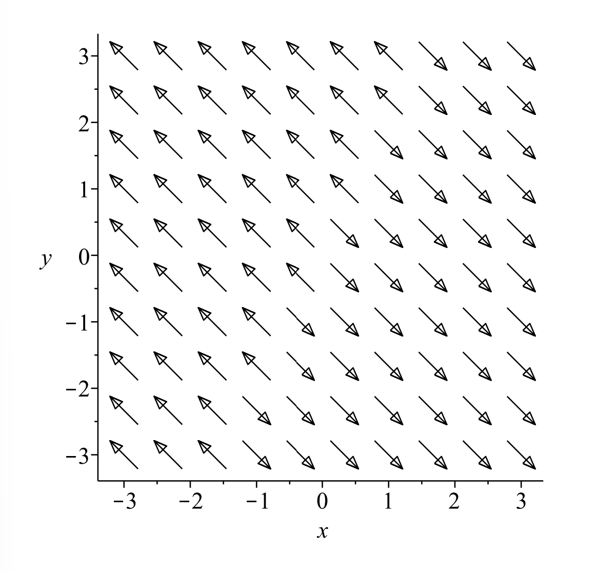
\[ \begin{aligned} &x^{\prime}=2 x-y \\ &y^{\prime}=-2 x+y \end{aligned} \label{6.29} \]
In this last example, we have a coupled set of equations. We rewrite it as a second order differential equation:
\[ \begin{aligned} x^{\prime \prime} &=2 x^{\prime}-y^{\prime} \\ &=2 x^{\prime}-(-2 x+y) \\ &=2 x^{\prime}+2 x+\left(x^{\prime}-2 x\right)=3 x^{\prime} \end{aligned} \label{6.30} \]
So, the second order equation is
\[x^{\prime \prime}-3 x^{\prime}=0 \nonumber \]
and the characteristic equation is \(0=r(r-3)\). This gives the general solution as
\[x(t)=c_{1}+c_{2} e^{3 t}\nonumber \]
and thus
\[y=2 x-x^{\prime}=2\left(c_{1}+c_{2} e^{3} t\right)-\left(3 c_{2} e^{3 t}\right)=2 c_{1}-c_{2} e^{3 t}\nonumber \]
In Figure 6.19 we show the direction field. The constant slope field seen in this example is confirmed by a simple computation:
\[\dfrac{d y}{d x}=\dfrac{-2 x+y}{2 x-y}=-1 .\nonumber \]
Furthermore, looking at initial conditions with \(y=2 x\), we have at \(t=0\),
\[2 c_{1}-c_{2}=2\left(c_{1}+c_{2}\right) \quad \Rightarrow \quad c_{2}=0\nonumber \]
Therefore, points on this line remain on this line forever, \((x, y)=\) \(\left(c_{1}, 2 c_{1}\right) .\) This line of fixed points is called a line of equilibria.
6.1.4: Polar Representation of Spirals
IN THE EXAMPLES WITH A CENTER OR A SPIRAL, one might be able to write the solutions in polar coordinates. Recall that a point in the plane can be described by either Cartesian \((x, y)\) or polar \((r, \theta)\) coordinates. Given the polar form, one can find the Cartesian components using
\[x=r \cos \theta \text { and } y=r \sin \theta \nonumber \]
Given the Cartesian coordinates, one can find the polar coordinates using
\[r^{2}=x^{2}+y^{2} \text { and } \tan \theta=\dfrac{y}{x} \nonumber \]
Since \(x\) and \(y\) are functions of \(t\), then naturally we can think of \(r\) and \(\theta\) as functions of \(t\). Converting a system of equations in the plane for \(x^{\prime}\) and \(y^{\prime}\) to polar form requires knowing \(r^{\prime}\) and \(\theta^{\prime} .\) So, we first find expressions for \(r^{\prime}\) and \(\theta^{\prime}\) in terms of \(x^{\prime}\) and \(y^{\prime}\).
Differentiating the first equation in Equation \(\PageIndex{31}\) gives
\[r r^{\prime}=x x^{\prime}+y y^{\prime}.\nonumber \]
Inserting the expressions for \(x^{\prime}\) and \(y^{\prime}\) from system \(\PageIndex{9}\), we have
\[r r^{\prime}=x(a x+b y)+y(c x+d y)\nonumber \]
In some cases this may be written entirely in terms of \(r^{\prime}\) s. Similarly, we have that
\[\theta^{\prime}=\dfrac{x y^{\prime}-y x^{\prime}}{r^{2}}\nonumber \]
which the reader can prove for homework.
In summary, when converting first order equations from rectangular to polar form, one needs the relations below.
Derivatives of Polar Variables
\[ \begin{aligned}r^{\prime} &=\dfrac{x x^{\prime}+y y^{\prime}}{r} \\\theta^{\prime} &=\dfrac{x y^{\prime}-y x^{\prime}}{r^{2}} \end{aligned} \label{6.32} \]
Rewrite the following system in the resulting system.
\[ \begin{aligned}x^{\prime} &=a x+b y \\y^{\prime} &=-b x+a y .\end{aligned}\label{6.33} \]
We first compute \(r^{\prime}\) and \(\theta^{\prime}\) :
\[r r^{\prime}=x x^{\prime}+y y^{\prime}=x(a x+b y)+y(-b x+a y)=a r^{2} \nonumber \]
\[r^{2} \theta^{\prime}=x y^{\prime}-y x^{\prime}=x(-b x+a y)-y(a x+b y)=-b r^{2} .\nonumber \]
This leads to simpler system
\[ \begin{aligned} r^{\prime} &=a r \\ \theta^{\prime} &=-b \end{aligned} \label{6.34} \]
This system is uncoupled. The second equation in this system indicates that we traverse the orbit at a constant rate in the clockwise direction. Solving these equations, we have that \(r(t)=r_{0} e^{a t}, \quad \theta(t)=\) \(\theta_{0}-b t\). Eliminating \(t\) between these solutions, we finally find the polar equation of the orbits:
\[r=r_{0} e^{-a\left(\theta-\theta_{0}\right) t / b} \nonumber \]
If you graph this for \(a \neq 0\), you will get stable or unstable spirals.
Consider the specific system
\[ \begin{aligned} &x^{\prime}=-y+x \\ &y^{\prime}=x+y \end{aligned} \label{6.35} \]
In order to convert this system into polar form, we compute
\[\begin{gathered} r r^{\prime}=x x^{\prime}+y y^{\prime}=x(-y+x)+y(x+y)=r^{2} \\ r^{2} \theta^{\prime}=-x y^{\prime}-y x^{\prime}=x(x+y)-y(-y+x)=r^{2} \end{gathered} \nonumber \]
This leads to simpler system
\[ \begin{aligned} &r^{\prime}=r \\ &\theta^{\prime}=1 . \end{aligned} \label{6.36} \]
Solving these equations yields
\[r(t)=r_{0} e^{t}, \quad \theta(t)=t+\theta_{0} \nonumber \]
Eliminating \(t\) from this solution gives the orbits in the phase plane, \(r(\theta)=r_{0} e^{\theta-\theta_{0}} .\)
A more complicated example arises for a nonlinear system of differential equations. Consider the following example.
\[ \begin{aligned} &x^{\prime}=-y+x\left(1-x^{2}-y^{2}\right) \\ &y^{\prime}=x+y\left(1-x^{2}-y^{2}\right) \end{aligned} \label{6.37} \]
Transforming to polar coordinates, one can show that in order to convert this system into polar form, we compute
\[r^{\prime}=r\left(1-r^{2}\right), \quad \theta^{\prime}=1 \nonumber \]
This uncoupled system can be solved and this is left to the reader.