Mathematics LibreTexts

6.6: Examples of the Matrix Method

  • Page ID
    91083
  • \( \newcommand{\vecs}[1]{\overset { \scriptstyle \rightharpoonup} {\mathbf{#1}} } \) \( \newcommand{\vecd}[1]{\overset{-\!-\!\rightharpoonup}{\vphantom{a}\smash {#1}}} \)\(\newcommand{\id}{\mathrm{id}}\) \( \newcommand{\Span}{\mathrm{span}}\) \( \newcommand{\kernel}{\mathrm{null}\,}\) \( \newcommand{\range}{\mathrm{range}\,}\) \( \newcommand{\RealPart}{\mathrm{Re}}\) \( \newcommand{\ImaginaryPart}{\mathrm{Im}}\) \( \newcommand{\Argument}{\mathrm{Arg}}\) \( \newcommand{\norm}[1]{\| #1 \|}\) \( \newcommand{\inner}[2]{\langle #1, #2 \rangle}\) \( \newcommand{\Span}{\mathrm{span}}\) \(\newcommand{\id}{\mathrm{id}}\) \( \newcommand{\Span}{\mathrm{span}}\) \( \newcommand{\kernel}{\mathrm{null}\,}\) \( \newcommand{\range}{\mathrm{range}\,}\) \( \newcommand{\RealPart}{\mathrm{Re}}\) \( \newcommand{\ImaginaryPart}{\mathrm{Im}}\) \( \newcommand{\Argument}{\mathrm{Arg}}\) \( \newcommand{\norm}[1]{\| #1 \|}\) \( \newcommand{\inner}[2]{\langle #1, #2 \rangle}\) \( \newcommand{\Span}{\mathrm{span}}\)\(\newcommand{\AA}{\unicode[.8,0]{x212B}}\)

    Here we will give some examples for typical systems for the three cases mentioned in the last section.

    Example \(\PageIndex{1}\)

    \(A=\left(\begin{array}{ll}4 & 2 \\ 3 & 3\end{array}\right)\).

    Eigenvalues: We first determine the eigenvalues.

    \[0=\left|\begin{array}{cc} 4-\lambda & 2 \\ 3 & 3-\lambda \end{array}\right| \nonumber \]

    Therefore,

    \[ \begin{aligned} 0 &=(4-\lambda)(3-\lambda)-6 \\ 0 &=\lambda^{2}-7 \lambda+6 \\ 0 &=(\lambda-1)(\lambda-6) \end{aligned} \label{6.72} \]

    The eigenvalues are then \(\lambda=1,6\). This is an example of Case I.

    Eigenvectors: Next we determine the eigenvectors associated with each of these eigenvalues. We have to solve the system \(A \mathbf{v}=\lambda \mathbf{v}\) in each case.

    Case \(\lambda=1\).

    \[\left(\begin{array}{ll} 4 & 2 \\ 3 & 3 \end{array}\right)\left(\begin{array}{l} v_{1} \\ v_{2} \end{array}\right)=\left(\begin{array}{l} v_{1} \\ v_{2} \end{array}\right) \nonumber \]

    \[\left(\begin{array}{ll} 3 & 2 \\ 3 & 2 \end{array}\right)\left(\begin{array}{l} v_{1} \\ v_{2} \end{array}\right)=\left(\begin{array}{l} 0 \\ 0 \end{array}\right) \nonumber \]

    This gives \(3 v_{1}+2 v_{2}=0 .\) One possible solution yields an eigenvector of

    \[\left(\begin{array}{l} v_{1} \\ v_{2} \end{array}\right)=\left(\begin{array}{c} 2 \\ -3 \end{array}\right) \nonumber \]

    Case \(\lambda=6\)

    \[\left(\begin{array}{cc} 4 & 2 \\ 3 & 3 \end{array}\right)\left(\begin{array}{l} v_{1} \\ v_{2} \end{array}\right)=6\left(\begin{array}{l} v_{1} \\ v_{2} \end{array}\right) \nonumber \]

    \[\left(\begin{array}{cc} -2 & 2 \\ 3 & -3 \end{array}\right)\left(\begin{array}{l} v_{1} \\ v_{2} \end{array}\right)=\left(\begin{array}{l} 0 \\ 0 \end{array}\right) \nonumber \]

    For this case we need to solve \(-2 v_{1}+2 v_{2}=0\). This yields

    \[\left(\begin{array}{l} v_{1} \\ v_{2} \end{array}\right)=\left(\begin{array}{l} 1 \\ 1 \end{array}\right)\nonumber \]

    General Solution: We can now construct the general solution.

    \[ \begin{aligned} \mathbf{x}(t) &=c_{1} e^{\lambda_{1} t} \mathbf{v}_{1}+c_{2} e^{\lambda_{2} t} \mathbf{v}_{2} \\ &=c_{1} e^{t}\left(\begin{array}{c} 2 \\ -3 \end{array}\right)+c_{2} e^{6 t}\left(\begin{array}{l} 1 \\ 1 \end{array}\right) \\ &=\left(\begin{array}{c} 2 c_{1} e^{t}+c_{2} e^{6 t} \\ -3 c_{1} e^{t}+c_{2} e^{6 t} \end{array}\right) \end{aligned} \label{6.78} \]

    Example \(\PageIndex{2}\)

    \(A=\left(\begin{array}{rr}3 & -5 \\ 1 & -1\end{array}\right)\).

    Eigenvalues: Again, one solves the eigenvalue equation.

    \[0=\left|\begin{array}{cc} 3-\lambda & -5 \\ 1 & -1-\lambda \end{array}\right| \nonumber \]

    Therefore,

    \[ \begin{aligned} 0 &=(3-\lambda)(-1-\lambda)+5 \\ 0 &=\lambda^{2}-2 \lambda+2 \\ \lambda &=\dfrac{-(-2) \pm \sqrt{4-4(1)(2)}}{2}=1 \pm i \end{aligned} \label{6.80} \]

    The eigenvalues are then \(\lambda=1+i, 1-i\). This is an example of Case III.

    Eigenvectors: In order to find the general solution, we need only find the eigenvector associated with \(1+i\).

    \[ \begin{aligned} \left(\begin{array}{cc} 3 & -5 \\ 1 & -1 \end{array}\right)\left(\begin{array}{l} v_{1} \\ v_{2} \end{array}\right) &=(1+i)\left(\begin{array}{l} v_{1} \\ v_{2} \end{array}\right) \\ \left(\begin{array}{cc} 2-i & -5 \\ 1 & -2-i \end{array}\right)\left(\begin{array}{l} v_{1} \\ v_{2} \end{array}\right) &=\left(\begin{array}{l} 0 \\ 0 \end{array}\right) \end{aligned} \label{6.81} \]

    We need to solve \((2-i) v_{1}-5 v_{2}=0\). Thus,

    \[\left(\begin{array}{l} v_{1} \\ v_{2} \end{array}\right)=\left(\begin{array}{c} 2+i \\ 1 \end{array}\right) \nonumber \]

    Complex Solution: In order to get the two real linearly independent solutions, we need to compute the real and imaginary parts of \(\mathbf{v} e^{\lambda t} .\)

    \[e^{\lambda t}\left(\begin{array}{c} 2+i \\ 1 \end{array}\right)=e^{(1+i) t}\left(\begin{array}{c} 2+i \\ 1 \end{array}\right) \nonumber \]

    \[\begin{aligned} &=e^{t}(\cos t+i \sin t)\left(\begin{array}{c} 2+i \\ 1 \end{array}\right) \\ &=e^{t}\left(\begin{array}{c} (2+i)(\cos t+i \sin t) \\ \cos t+i \sin t \end{array}\right) \\ &=e^{t}\left(\begin{array}{c} (2 \cos t-\sin t)+i(\cos t+2 \sin t) \\ \cos t+i \sin t \end{array}\right) \\ &=e^{t}\left(\begin{array}{c} 2 \cos t-\sin t \\ \cos t \end{array}\right)+i e^{t}\left(\begin{array}{c} \cos t+2 \sin t \\ \sin t \end{array}\right) \end{aligned} \nonumber \]

    General Solution: Now we can construct the general solution.

    \[\begin{aligned} \mathbf{x}(t) &=c_{1} e^{t}\left(\begin{array}{l} 2 \cos t-\sin t \\ \cos t \end{array}\right)+c_{2} e^{t}\left(\begin{array}{c} \cos t+2 \sin t \\ \sin t \end{array}\right) \\ &=e^{t}\left(\begin{array}{c} c_{1}(2 \cos t-\sin t)+c_{2}(\cos t+2 \sin t) \\ c_{1} \cos t+c_{2} \sin t \end{array}\right) \end{aligned} \nonumber \]

    Note: This can be rewritten as

    \[\mathbf{x}(t)=e^{t} \cos t\left(\begin{array}{c} 2 c_{1}+c_{2} \\ c_{1} \end{array}\right)+e^{t} \sin t\left(\begin{array}{c} 2 c_{2}-c_{1} \\ c_{2} \end{array}\right) \nonumber \]

    Example \(\PageIndex{3}\)

    \(A=\left(\begin{array}{cc}7 & -1 \\ 9 & 1\end{array}\right)\).

    Eigenvalues:

    \[0=\left|\begin{array}{cc} 7-\lambda & -1 \\ 9 & 1-\lambda \end{array}\right| \nonumber \]

    Therefore,

    \[ \begin{aligned} 0 &=(7-\lambda)(1-\lambda)+9 \\ 0 &=\lambda^{2}-8 \lambda+16 \\ 0 &=(\lambda-4)^{2} \end{aligned} \label{6.85} \]

    There is only one real eigenvalue, \(\lambda=4\). This is an example of Case II.

    Eigenvectors: In this case we first solve for \(\mathbf{v}_{1}\) and then get the second linearly independent vector.

    \[ \begin{aligned} &\left(\begin{array}{cc} 7 & -1 \\ 9 & 1 \end{array}\right)\left(\begin{array}{l} v_{1} \\ v_{2} \end{array}\right)=4\left(\begin{array}{l} v_{1} \\ v_{2} \end{array}\right) \\ &\left(\begin{array}{cc} 3 & -1 \\ 9 & -3 \end{array}\right)\left(\begin{array}{l} v_{1} \\ v_{2} \end{array}\right)=\left(\begin{array}{l} 0 \\ 0 \end{array}\right) \end{aligned} \label{6.86} \]

    Therefore, we have

    \[3 v_{1}-v_{2}=0, \quad \Rightarrow \quad\left(\begin{array}{l} v_{1} \\ v_{2} \end{array}\right)=\left(\begin{array}{l} 1 \\ 3 \end{array}\right) \nonumber \]

    Second Linearly Independent Solution: Now we need to solve \(A \mathbf{v}_{2}-\lambda \mathbf{v}_{2}=\mathbf{v}_{1}\).

    \[ \begin{aligned} \left(\begin{array}{cc} 7 & -1 \\ 9 & 1 \end{array}\right)\left(\begin{array}{l} u_{1} \\ u_{2} \end{array}\right)-4\left(\begin{array}{l} u_{1} \\ u_{2} \end{array}\right) &=\left(\begin{array}{l} 1 \\ 3 \end{array}\right) \\ \left(\begin{array}{ll} 3 & -1 \\ 9 & -3 \end{array}\right)\left(\begin{array}{l} u_{1} \\ u_{2} \end{array}\right) &=\left(\begin{array}{l} 1 \\ 3 \end{array}\right) \end{aligned} \label{6.87} \]

    Expanding the matrix product, we obtain the system of equations

    \[ \begin{aligned} 3 u_{1}-u_{2} &=1 \\ 9 u_{1}-3 u_{2} &=3 \end{aligned}\label{6.88} \]

    The solution of this system is \(\left(\begin{array}{l}u_{1} \\ u_{2}\end{array}\right)=\left(\begin{array}{l}1 \\ 2\end{array}\right)\).

    General Solution: We construct the general solution as

    \[ \begin{aligned} \mathbf{y}(t) &=c_{1} e^{\lambda t} \mathbf{v}_{1}+c_{2} e^{\lambda t}\left(\mathbf{v}_{2}+t \mathbf{v}_{1}\right) \\ &=c_{1} e^{4 t}\left(\begin{array}{c} 1 \\ 3 \end{array}\right)+c_{2} e^{4 t}\left[\left(\begin{array}{l} 1 \\ 2 \end{array}\right)+t\left(\begin{array}{l} 1 \\ 3 \end{array}\right)\right] \\ &=e^{4 t}\left(\begin{array}{c} c_{1}+c_{2}(1+t) \\ 3 c_{1}+c_{2}(2+3 t) \end{array}\right) \end{aligned} \label{6.89} \]

    6.6.1: Planar Systems - Summary

    The reader should have noted by now that there is a connection between the behavior of the solutions obtained in Section 6.1.3 and the eigenvalues found from the coefficient matrices in the previous examples. In Table \(6.2\) we summarize some of these cases.

    Table \(\PageIndex{1}\): List of typical behaviors in planar systems.
    Type Eigenvalues Stability
    Node Real \(\lambda\), same signs

    \(\lambda<0\), stable

    \(\lambda>0\), unstable

    Saddle Real \(\lambda\) opposite signs Mostly Unstable
    Center \(\lambda\) pure imaginary \(-\)
    Focus/Spiral Complex \(\lambda, \operatorname{Re}(\lambda) \neq 0\)

    \(\operatorname{Re}(\lambda)<0\), stable

    \(\operatorname{Re}(\lambda)>0\), unstable

    Degenerate Node Repeated roots, \(\lambda>0\), stable
    Lines of Equilibria One zero eigenvalue \(\lambda<0\), stable

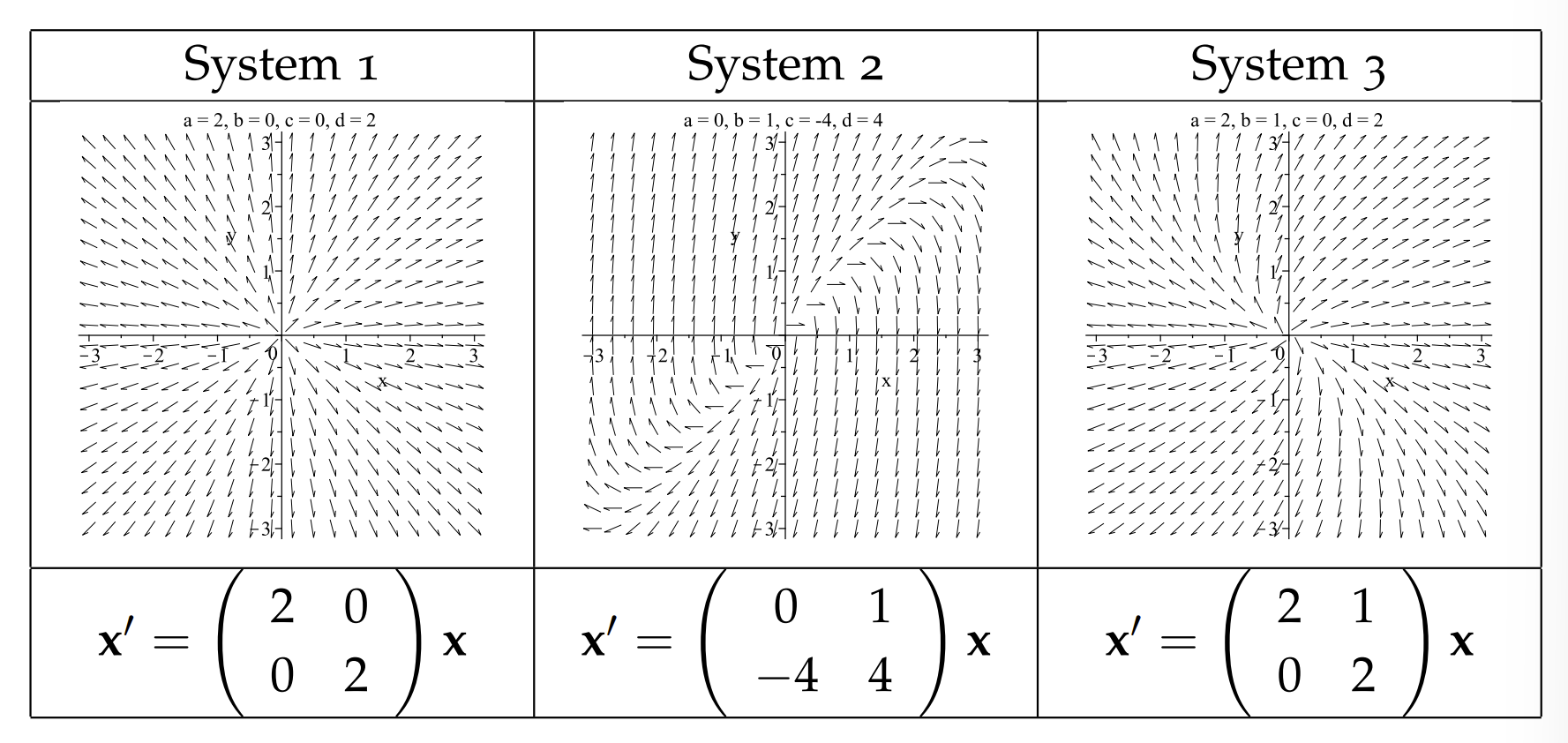
    The connection, as we have seen, is that the characteristic equation for the associated second order differential equation is the same as the eigenvalue equation of the coefficient matrix for the linear system. However, one should be a little careful in cases in which the coefficient matrix in not diagonalizable. In Table \(6.3\) are three examples of systems with repeated roots. The reader should look at these systems and look at the commonalities and differences in these systems and their solutions. In these cases one has unstable nodes, though they are degenerate in that there is only one accessible eigenvector.

    clipboard_ec4008bcb12679c969b97c7eb6f5d1022.png
    Figure \(\PageIndex{1}\): Three examples of systems with a repeated root of \(\lambda=2\).

    Another way to look at the classification of these solution is to use the determinant and trace of the coefficient matrix. Recall that the determinant and trace of \(A=\left(\begin{array}{ll}a & b \\ c & d\end{array}\right)\) are given by \(\operatorname{det} A=a d-b c\) and \(\operatorname{tr} A=a+d\)

    We note that the general eigenvalue equation,

    \[\lambda^{2}-(a+d) \lambda+a d-b c=0 \nonumber \]

    can be written as

    \[\lambda^{2}-(\operatorname{tr} A) \lambda+\operatorname{det} A=0 \nonumber \]

    Therefore, the eigenvalues are found from the quadratic formula as

    \[\lambda_{1,2}=\dfrac{\operatorname{tr} A \pm \sqrt{(\operatorname{tr} A)^{2}-4 \operatorname{det} A}}{2} \nonumber \]

    The solution behavior then depends on the sign of discriminant,

    \[(\operatorname{tr} A)^{2}-4 \operatorname{det} A \nonumber \]

    If we consider a plot of where the discriminant vanishes, then we could plot

    \[(\operatorname{tr} A)^{2}=4 \operatorname{det} A \nonumber \]

    in the \(\operatorname{det} A \operatorname{tr} A\) )-plane. This is a parabolic cure as shown by the dashed line in Figure \(6.25\). The region inside the parabola have a negative discriminant, leading to complex roots. In these cases we have oscillatory solutions. If \(\operatorname{tr} A=0\), then one has centers. If \(\operatorname{tr} A<0\), the solutions are stable spirals; otherwise, they are unstable spirals. If the discriminant is positive, then the roots are real, leading to nodes or saddles in the regions indicated.


    This page titled 6.6: Examples of the Matrix Method is shared under a CC BY-NC-SA 3.0 license and was authored, remixed, and/or curated by Russell Herman via source content that was edited to the style and standards of the LibreTexts platform; a detailed edit history is available upon request.