6.9: Problems

1. Consider the system

\[\begin{gathered} x^{\prime}=-4 x-y \\ y^{\prime}=x-2 y \end{gathered} \nonumber \]

1. Determine the second order differential equation satisfied by \(x(t)\).
2. Solve the differential equation for \(x(t)\).
3. Using this solution, find \(y(t)\).
4. Verify your solutions for \(x(t)\) and \(y(t)\).
5. Find a particular solution to the system given the initial conditions \(x(0)=1\) and \(y(0)=0\).

2. Consider the following systems. Determine the families of orbits for each system and sketch several orbits in the phase plane and classify them by their type (stable node, etc.)
   1. \[\begin{aligned} &x^{\prime}=3 x \\ &y^{\prime}=-2 y . \end{aligned} \nonumber \]

   2. \[\begin{aligned} &x^{\prime}=-y \\ &y^{\prime}=-5 x \end{aligned} \nonumber \]

   3. \[\begin{aligned} &x^{\prime}=2 y \\ &y^{\prime}=-3 x \end{aligned} \nonumber \]

   4. \[\begin{aligned} &x^{\prime}=x-y \\ &y^{\prime}=y . \end{aligned} \nonumber \]

   5. \[\begin{aligned} x^{\prime} &=2 x+3 y \\ y^{\prime} &=-3 x+2 y \end{aligned} \nonumber \]

3. Use the transformations relating polar and Cartesian coordinates to prove that

\[\dfrac{d \theta}{d t}=\dfrac{1}{r^{2}}\left[x \dfrac{d y}{d t}-y \dfrac{d x}{d t}\right]\nonumber \]

4. Consider the system of equations in Example 6.1.13.
   1. Derive the polar form of the system.
   2. Solve the radial equation, \(r^{\prime}=r\left(1-r^{2}\right)\), for the initial values \(r(0)=0,0.5,1.0,2.0 .\)
   3. Based upon these solutions, plot and describe the behavior of all solutions to the original system in Cartesian coordinates.
5. Consider the following systems. For each system determine the coefficient matrix. When possible, solve the eigenvalue problem for each matrix and use the eigenvalues and eigenfunctions to provide solutions to the given systems. Finally, in the common cases which you investigated in Problem 2, make comparisons with your previous answers, such as what type of eigenvalues correspond to stable nodes.
   1. \[\begin{aligned} &x^{\prime}=3 x-y \\ &y^{\prime}=2 x-2 y \end{aligned} \nonumber \]

   2. \[\begin{aligned} &x^{\prime}=-y \\ &y^{\prime}=-5 x \end{aligned} \nonumber \]

   3. \[\begin{aligned} x^{\prime} &=x-y \\ y^{\prime} &=y . \end{aligned} \nonumber \]

   4. \[\begin{aligned} &x^{\prime}=2 x+3 y \\ &y^{\prime}=-3 x+2 y . \end{aligned} \nonumber \]

   5. \[\begin{aligned} &x^{\prime}=-4 x-y \\ &y^{\prime}=x-2 y \end{aligned} \nonumber \]

   6. \[\begin{aligned} &x^{\prime}=x-y \\ &y^{\prime}=x+y \end{aligned} \nonumber \]

6. For the given matrix, evaluate \(e^{t A}\), using the definition

\[e^{t A}=\sum_{n=0}^{\infty} \dfrac{t^{n}}{n !} A^{n}=I+t A+\dfrac{t^{2}}{2} A^{2}+\dfrac{t^{3}}{3 !} A^{3}+\ldots\nonumber \]

and simplifying.

1. \(A=\left(\begin{array}{ll}1 & 0 \\ 0 & 2\end{array}\right)\)
2. \(A=\left(\begin{array}{cc}1 & 0 \\ -2 & 2\end{array}\right)\).
3. \(A=\left(\begin{array}{cc}0 & -1 \\ 0 & 1\end{array}\right)\).
4. \(A=\left(\begin{array}{ll}0 & 1 \\ 1 & 0\end{array}\right)\)
5. \(A=\left(\begin{array}{cc}0 & -i \\ i & 0\end{array}\right)\).
6. \(A=\left(\begin{array}{lll}0 & 1 & 0 \\ 0 & 0 & 1 \\ 0 & 0 & 0\end{array}\right)\)

7. Find the fundamental matrix solution for the system \(\mathbf{x}^{\prime}=A \mathbf{x}\) where matrix \(A\) is given. If an initial condition is provided, find the solution of the initial value problem using the principal matrix.
   1. \(A=\left(\begin{array}{cc}1 & 0 \\ -2 & 2\end{array}\right)\)
   2. \(A=\left(\begin{array}{cc}12 & -15 \\ 4 & -4\end{array}\right), \mathbf{x}(0)=\left(\begin{array}{l}1 \\ 0\end{array}\right)\)
   3. \(A=\left(\begin{array}{rr}2 & -1 \\ 5 & -2\end{array}\right)\).
   4. \(A=\left(\begin{array}{cc}4 & -13 \\ 2 & -6\end{array}\right), \mathbf{x}(0)=\left(\begin{array}{l}2 \\ 0\end{array}\right)\)
   5. \(A=\left(\begin{array}{ll}4 & 2 \\ 3 & 3\end{array}\right)\)
   6. \(A=\left(\begin{array}{cc}3 & 5 \\ -1 & 1\end{array}\right)\)
   7. \(A=\left(\begin{array}{cc}8 & -5 \\ 16 & 8\end{array}\right), \mathbf{x}(0)=\left(\begin{array}{c}1 \\ -1\end{array}\right)\)
   8. \(A=\left(\begin{array}{ll}1 & -2 \\ 2 & -3\end{array}\right)\).
   9. \(A=\left(\begin{array}{lll}5 & 4 & 2 \\ 4 & 5 & 2 \\ 2 & 2 & 2\end{array}\right)\)
8. Solve the following initial value problems using Equation 6.8.6, the solution of a nonhomogeneous system using the principal matrix solution.
   1. \[\mathbf{x}^{\prime}=\left(\begin{array}{cc} 2 & -1 \\ 3 & -2 \end{array}\right) \mathbf{x}+\left(\begin{array}{c} e^{t} \\ t \end{array}\right), \mathbf{x}(0)=\left(\begin{array}{l} 1 \\ 2 \end{array}\right) \nonumber \]

   2. \[\mathbf{x}^{\prime}=\left(\begin{array}{cc} 5 & 3 \\ -6 & -4 \end{array}\right) \mathbf{x}+\left(\begin{array}{c} 1 \\ e^{t} \end{array}\right), \mathbf{x}(0)=\left(\begin{array}{l} 1 \\ 0 \end{array}\right) \nonumber \]

   3. \[\mathbf{x}^{\prime}=\left(\begin{array}{cc} 2 & -1 \\ 5 & -2 \end{array}\right) \mathbf{x}+\left(\begin{array}{c} \cos t \\ \sin t \end{array}\right), \mathbf{x}(0)=\left(\begin{array}{l} 0 \\ 1 \end{array}\right) \nonumber \]

9. Add a third spring connected to mass two in the coupled system shown in Figure 6.1.2 to a wall on the far right. Assume that the masses are the same and the springs are the same.
   1. Model this system with a set of first order differential equations.
   2. If the masses are all \(2.0 \mathrm{~kg}\) and the spring constants are all \(10.0\) \(\mathrm{N} / \mathrm{m}\), then find the general solution for the system.
   3. Move mass one to the left (of equilibrium) \(10.0 \mathrm{~cm}\) and mass two to the right \(5.0 \mathrm{~cm}\). Let them go. find the solution and plot it as a function of time. Where is each mass at \(5.0\) seconds?
   4. Model this initial value problem with a set of two second order differential equations. Set up the system in the form \(M \ddot{\mathbf{x}}=-K \mathbf{x}\) and solve using the values in part \(b\).
10. In Example 6.1.14 we investigated a couple mass-spring system as a pair of second order differential equations.
    1. In that problem we used \(\sqrt{\dfrac{3 \pm \sqrt{5}}{2}}=\dfrac{\sqrt{5} \pm 1}{2}\). Prove this result.
    2. Rewrite the system as a system of four first order equations.
    3. Find the eigenvalues and eigenfunctions for the system of equations in part b to arrive at the solution found in Example 6.1.14.
    4. Let \(k=5.00 \mathrm{~N} / \mathrm{m}\) and \(m=0.250 \mathrm{~kg}\). Assume that the masses are initially at rest and plot the positions as a function of time if initially i) \(x_{1}(0)=x_{2}(0)=10.0 \mathrm{~cm}\) and i) \(x_{1}(0)=-x_{2}(0)=10.0\) \(\mathrm{cm}\). Describe the resulting motion.
11. Consider the series circuit in Figure \(2.4\) with \(L=1.00 \mathrm{H}, R=1.00 \times 10^{2}\) \(\Omega, C=1.00 \times 10^{-4} \mathrm{~F}\), and \(V_{0}=1.00 \times 10^{3} \mathrm{~V}\)
    1. Set up the problem as a system of two first order differential equations for the charge and the current.
    2. Suppose that no charge is present and no current is flowing at time \(t=0\) when \(V_{0}\) is applied. Find the current and the charge on the capacitor as functions of time.
    3. Plot your solutions and describe how the system behaves over time.
12. Consider the series circuit in Figure 6.2.2.1 with \(L=1.00 \mathrm{H}, R_{1}=R_{2}=\) \(1.00 \times 10^{2} \Omega, C=1.00 \times 10^{-4} \mathrm{~F}\), and \(V_{0}=1.00 \times 10^{3} \mathrm{~V}\).
    1. Set up the problem as a system of first order differential equations for the charges and the currents in each loop.
    2. Suppose that no charge is present and no current is flowing at time \(t=0\) when \(V_{0}\) is applied. Find the current and the charge on the capacitor as functions of time.
    3. Plot your solutions and describe how the system behaves over time.
13. Initially a 100 gallon tank is filled with pure water. At time \(t=0\) water with a half a pound of salt per two gallons is added to the container at the rate of 3 gallons per minute, and the well-stirred mixture is drained from the container at the same rate.
    1. Find the number of pounds of salt in the container as a function of time.
    2. How many minutes does it take for the concentration to reach 2 pounds per gallon?
    3. What does the concentration in the container approach for large values of time? Does this agree with your intuition?
14. You make two quarts of salsa for a party. The recipe calls for five teaspoons of lime juice per quart, but you had accidentally put in five tablespoons per quart. You decide to feed your guests the salsa anyway. Assume that the guests take a quarter cup of salsa per minute and that you replace what was taken with chopped tomatoes and onions without any lime juice. [ 1 quart \(=4\) cups and \(1 \mathrm{~Tb}=3 \mathrm{tsp} .]\)
    1. Write down the differential equation and initial condition for the amount of lime juice as a function of time in this mixture-type problem.
    2. Solve this initial value problem.
    3. How long will it take to get the salsa back to the recipe’s suggested concentration?
15. Consider the chemical reaction leading to the system in Equations 6.2.4.3. Let the rate constants be \(k_{1}=0.20 \mathrm{~ms}^{-1}, k_{2}=0.05 \mathrm{~ms}^{-1}\), and \(k_{3}=0.10 \mathrm{~ms}^{-1}\). What do the eigenvalues of the coefficient matrix say about the behavior of the system? Find the solution of the system assuming \([A](0)=A_{0}=1.0\) \(\mu \mathrm{mol},[B](0)=0\), and \([C](0)=0 .\) Plot the solutions for \(t=0.0\) to \(50.0 \mathrm{~ms}\) and describe what is happening over this time.
16. Find and classify any equilibrium points in the Romeo and Juliet problem for the following cases. Solve the systems and describe their affections as a function of time.
    1. \(a=0, b=2, c=-1, d=0, R(0)=1, J(0)=1\).
    2. \(a=0, b=2, c=1, d=0, R(0)=1, J(0)=1\).
    3. \(a=-1, b=2, c=-1, d=0, R(0)=1, J(0)=1\).

Figure \(\PageIndex{1}\): Figure for Problem 17.

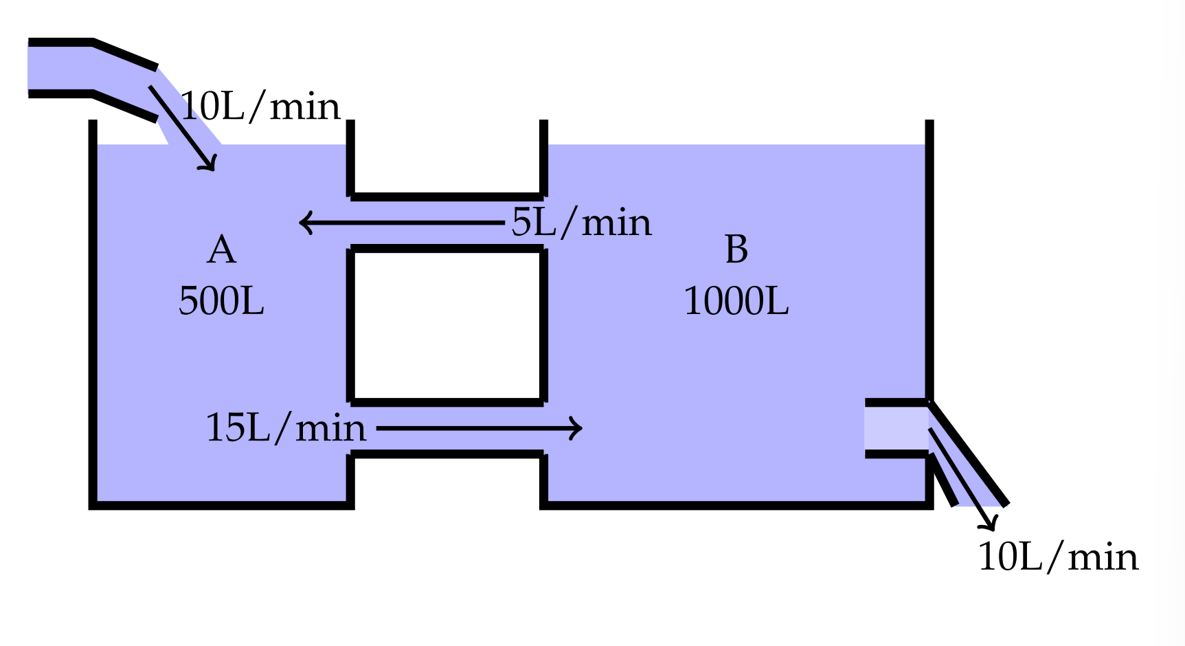
17. Two tanks contain a mixture of water and alcohol with tank A containing \(500 \mathrm{~L}\) and tank \(\mathrm{B}\) 1000 L. Initially, the concentration of alcohol in Tank \(\mathrm{A}\) is \(\mathrm{o} \%\) and that of \(\operatorname{tank} \mathrm{B}\) is \(8 \mathrm{o} \%\). Solution leaves \(\operatorname{tank} \mathrm{A}\) into \(\mathrm{B}\) at a rate of 15 liter/min and the solution in tank B returns to A at a rate of \(5 \mathrm{~L} / \mathrm{min}\) while well mixed solution also leaves the system at 10 liter/min through an outlet. A mixture of water and alcohol enters \(\operatorname{tank} A\) at the rate of 10 liter/min with the concentration of \(10 \%\) through an inlet. What will be the concentration of the alcohol of the solution in each tank after 10 mins?
18. Consider the tank system in Problem 17. Add a third \(\operatorname{tank}(C)\) to \(\tan \mathrm{k} B\) with a volume of \(300 \mathrm{~L}\). Connect \(C\) with \(8 \mathrm{~L} / \mathrm{min}\) from \(\operatorname{tank} \mathrm{B}\) and \(2 \mathrm{~L} / \mathrm{min}\) flow back. Let io \(\mathrm{L} / \mathrm{min}\) flow out of the system. If the initial concentration is \(10 \%\) in each tank and a mixture of water and alcohol enters tank \(A\) at the rate of 10 liter/min with the concentration of \(20 \%\) through an inlet, what will be the concentration of the alcohol in each of the tanks after an hour?
19. Consider the epidemic model leading to the system in Equation 6.2.7.1. Choose the constants as \(a=2.0\) days \(^{-1}, d=3.0\) days \(^{-1}\), and \(r=1.0\) days \(^{-1}\). What are the eigenvalues of the coefficient matrix? Find the solution of the system assuming an initial population of 1,000 and one infected individual. Plot the solutions for \(t=0.0\) to \(5.0\) days and describe what is happening over this time. Is this model realistic?