7.4: Bifurcations for First Order Equations

We now consider families of first order autonomous differential equations of the form

\[\dfrac{d y}{d t}=f(y ; \mu) \nonumber \]

Here \(\mu\) is a parameter that we can change and then observe the resulting behaviors of the solutions of the differential equation. When a small change in the parameter leads to changes in the behavior of the solution, then the system is said to undergo a bifurcation. The value of the parameter, \(\mu\), at which the bifurcation occurs is called a bifurcation point.

We will consider several generic examples, leading to special classes of bifurcations of first order autonomous differential equations. We will study the stability of equilibrium solutions using both phase lines and the stability criteria developed in the last section

Example \(\PageIndex{1}\)

\(y^{\prime}=y^{2}-\mu\).

Solution

First note that equilibrium solutions occur for \(y^{2}=\mu .\) In this problem, there are three cases to consider.

1. \(\mu>0\).

In this case there are two real solutions of \(y^{2}=\mu, y=\pm \sqrt{\mu}\). Note that \(y^{2}-\mu<0\) for \(|y|<\sqrt{\mu}\). So, we have the right phase line in Figure \(\PageIndex{1}\)\).

Figure \(\PageIndex{1}\): Phase lines for \(y^{\prime}=y^{2}-\mu\).On the right \(\mu>0\) and on the left \(\mu<0\).

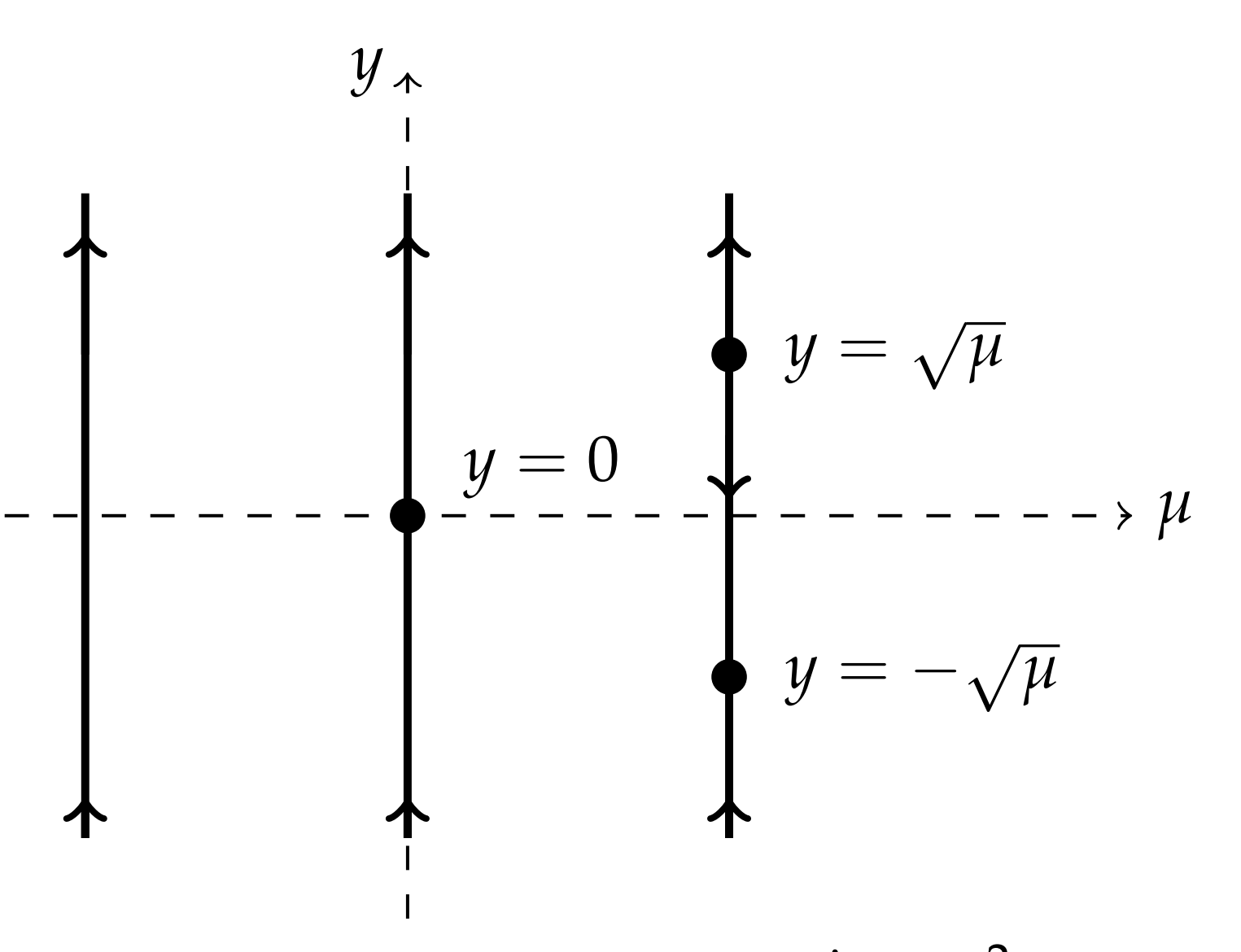
2. \( \mu = 0\).

There is only one equilibrium point at \(y=0\). The equation becomes \(y^{\prime}=y^{2} .\) It is obvious that the right side of this equation is never negative. So, the phase line, which is shown as the middle line in Figure \(\PageIndex{1}\), has upward pointing arrows.

3. \(\mu<0\).

In this case there are no equilibrium solutions. Since \(y^{2}-\mu>0\), the slopes for all solutions are positive as indicated by the last phase line in Figure \(\PageIndex{1}\).

We can also confirm the behaviors of the equilibrium points by noting that \(f^{\prime}(y)=2 y .\) Then, \(f^{\prime}(\pm \sqrt{\mu})=\pm 2 \sqrt{\mu}\) for \(\mu \geq 0 .\) Therefore, the equilibria \(y=+\sqrt{\mu}\) are unstable equilibria for \(\mu>0 .\) Similarly, the equilibria \(y=-\sqrt{\mu}\) are stable equilibria for \(\mu>0\).

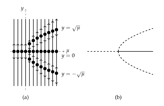
We can combine these results for the phase lines into one diagram known as a bifurcation diagram. We will plot the equilibrium solutions and their phase lines \(y=\pm \sqrt{\mu}\) in the \(\mu y\)-plane. We begin by lining up the phase lines for various \(\mu^{\prime}\) s. These are shown on the left side of Figure \(7.6\). Note the pattern of equilibrium points lies on the parabolic curve \(y^{2}=\mu\). The upper branch of this curve is a collection of unstable equilibria and the bottom is a stable branch. So, we can dispose of the phase lines and just keep the equilibria. However, we will draw the unstable branch as a dashed line and the stable branch as a solid line.

Figure \(\PageIndex{2}\): (a) The typical phase lines for \(y' = y^2 − \mu\). (b) Bifurcation diagram for \(y' = y^2 − \mu\). This is an example of a saddle-node bifurcation.

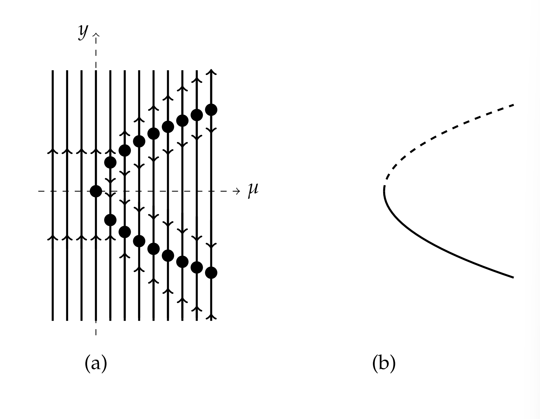
The bifurcation diagram is displayed on the right side of Figure \(\PageIndex{2}\). This type of bifurcation is called a saddle-node bifurcation. The point \(\mu=0\) at which the behavior changes is the bifurcation point. As \(\mu\) changes from negative to positive values, the system goes from having no equilibria to having one stable and one unstable equilibrium point.

Example \(\PageIndex{2}\)

\(y^{\prime}=y^{2}-\mu y\).

Solution

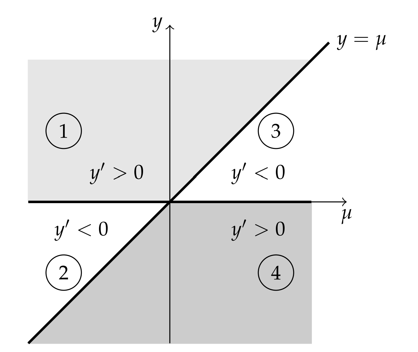
Writing this equation in factored form, \(y^{\prime}=y(y-\mu)\), we see that there are two equilibrium points, \(y=0\) and \(y=\mu\). The behavior of the solutions depends upon the sign of \(y^{\prime}=y(y-\mu)\). This leads to four cases with the indicated signs of the derivative. The regions indicating the signs of \(y^{\prime}\) are shown in Figure \(7 \cdot 7\).

1. \(y>0, y-\mu>0 \Rightarrow y^{\prime}>0\).
2. \(y<0, y-\mu>0 \Rightarrow y^{\prime}<0\).
3. \(y>0, y-\mu<0 \Rightarrow y^{\prime}<0\).
4. \(y<0, y-\mu<0 \Rightarrow y^{\prime}>0\).

Figure \(\PageIndex{3}\): The regions indicating the different signs of the derivative for \(y^{\prime}=\) \(y^{2}-\mu y\).

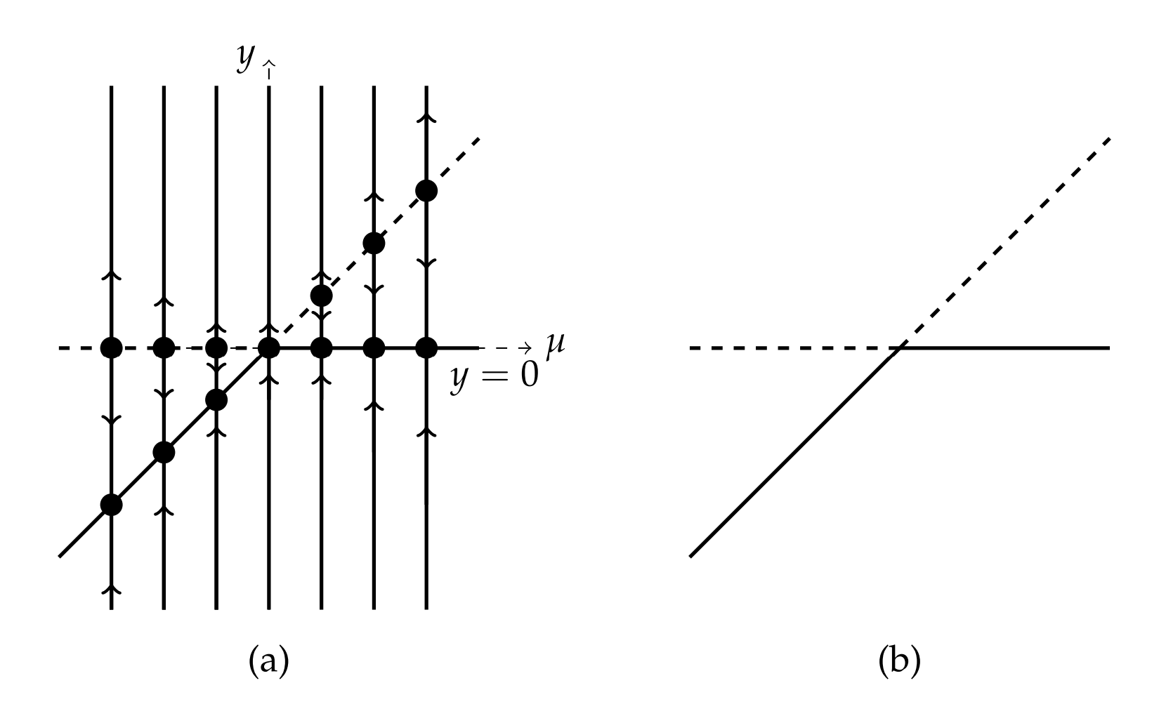
The corresponding phase lines and superimposed bifurcation diagram are shown in figure \(7.8\). The bifurcation diagram is on the right side of Figure \(7.8\) and this type of bifurcation is called a transcritical bifurcation.

Again, the stability can be determined from the derivative \(f^{\prime}(y)=\) \(2 y-\mu\) evaluated at \(y=0, \mu\). From \(f^{\prime}(0)=-\mu\), we see that \(y=0\) is stable for \(\mu>0\) and unstable for \(\mu<0\). Similarly, \(f^{\prime}(\mu)=\mu\) implies that \(y=\mu\) is unstable for \(\mu>0\) and stable for \(\mu<0 .\) These results are consistent with the phase line plots.

Example \(\PageIndex{3}\)

\(y^{\prime}=y^{3}-\mu y\).

Solution

For this last example, we find from \(y^{3}-\mu y=y\left(y^{2}-\mu\right)=0\) that there are two cases.

1. \(\mu<0 .\) In this case there is only one equilibrium point at \(y=0 .\) For positive values of \(y\) we have that \(y^{\prime}>0\) and for negative values of \(y\) we have that \(y^{\prime}<0\). Therefore, this is an unstable equilibrium point.

Figure \(\PageIndex{4}\): (a) Collection of phase lines for \(y^{\prime}=y^{2}-\mu y\). (b) Bifurcation diagram for \(y^{\prime}=y^{2}-\mu y\). This is an example of a transcritical bifurcation.

Figure \(\PageIndex{5}\): (a) The phase lines for \(y^{\prime}=\) \(y^{3}-\mu y\). The left one corresponds to \(\mu<\) 0 and the right phase line is for \(\mu>0\). (b) Bifurcation diagram for \(y^{\prime}=y^{3}-\mu y\). This is an example of a pitchfork bifurcation.

When two of the prongs of the pitchfork are unstable branches, the bifurcation is called a subcritical pitchfork bifurcation. When two prongs are stable branches, the bifurcation is a supercritical pitchfork bifurcation.

2. \(\mu>0 .\) Here we have three equilibria, \(y=0, \pm \sqrt{\mu} .\) A careful investigation shows that \(y=0\) is a stable equilibrium point and that the other two equilibria are unstable.

In Figure \(\PageIndex{5}\)\) we show the phase lines for these two cases. The corresponding bifurcation diagram is then sketched on the right side of Figure \(\PageIndex{5}\). For obvious reasons this has been labeled a pitchfork bifurcation.

Since \(f^{\prime}(y)=3 y^{2}-\mu\), the stability analysis gives that \(f^{\prime}(0)=-\mu .\) So, \(y=0\) is stable for \(\mu>0\) and unstable for \(\mu<0 .\) For \(\mu>0\), we have that \(f^{\prime}(\pm \sqrt{\mu})=2 \mu\). Therefore, \(y=\pm \sqrt{\mu}, \mu>0\), is unstable. Thus, we have a subcritical pitchfork bifurcation.