3.7: Nonlinear Population Models

We have already encountered several models of population dynamics. Of course, one could dream up several other examples. There are two standard types of models: Predator-prey and competing species. In the predator-prey model, one typically has one species, the predator, feeding on the other, the prey. We will look at the standard Lotka-Volterra model in this section. The competing species model looks similar, except there are a few sign changes, since one species is not feeding on the other. Also, we can build in logistic terms into our model. We will save this latter type of model for the homework.

The Lotka-Volterra model takes the form

\[\begin{aligned}
\dot{x} &= ax -bxy, \\
\dot{y} &= -dy + cxy
\end{aligned} \label{3.34} \]

In this case, we can think of \(x\) as the population of rabbits (prey) and \(y\) is the population of foxes (predators). Choosing all constants to be positive, we can describe the terms.

• \(ax\): When left alone, the rabbit population will grow. Thus \(a\) is the natural growth rate without predators.
• \(-dy\): When there no rabbits, the fox population should decay. Thus, the coefficient needs to be negative.

Figure 3.16. Phase plane for the damped nonlinear pendulum. Solution curves are shown for initial conditions \((x_0, y_0) = (0, 3), (0, 2), (0, 1), (5, 1)\).

• \(-b x y\) : We add a nonlinear term corresponding to the depletion of the rabbits when the foxes are around.
• \(cxy\): The more rabbits there are, the more food for the foxes. So, we add a nonlinear term giving rise to an increase in fox population.

The analysis of the Lotka-Volterra model begins with determining the fixed points. So, we have from Equation (3.34)

\[\begin{gathered}
x(a-b y)=0 \\
y(-d+c x)=0 .
\end{gathered} \label{3.35} \]

Therefore, the origin and \(\left(\dfrac{d}{c} \dfrac{a}{b}\right)\) are the fixed points.
Next, we determine their stability, by linearization about the fixed points. We can use the Jacobian matrix, or we could just expand the right hand side of each equation in (3.34). The Jacobian matrix is \(D f(x, y)=\left(\begin{array}{cc}a-b y & -b x \\ c y & -d+c x\end{array}\right)\).

Evaluating at each fixed point, we have

\[\begin{aligned}
D f(0,0) &=\left(\begin{array}{cc}
a & 0 \\
0 & -d
\end{array}\right)
\end{aligned} \label{3.36} \]

\[\begin{aligned}
D f\left(\dfrac{d}{c}, \dfrac{a}{b}\right) &=\left(\begin{array}{cc}
0 & -\dfrac{b d}{c} \\
\dfrac{a c}{b} & 0
\end{array}\right) .
\end{aligned} \label{3.37} \]

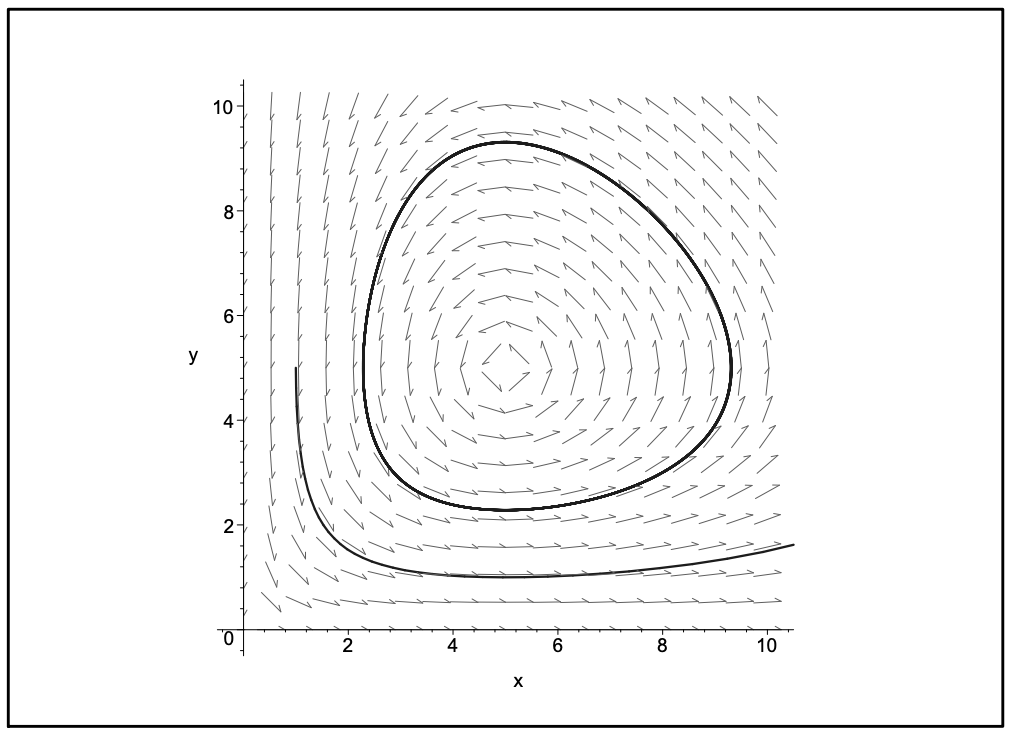
The eigenvalues of (3.36) are \(\lambda = a,-d\). So, the origin is a saddle point. The eigenvalues of (3.37) satisfy \(\lambda^2 + ad = 0\). So, the other point is a center. In Figure 3.17 we show a sample direction field for the Lotka-Volterra system.

Another way to linearize is to expand the equations about the fixed points. Even though this is equivalent to computing the Jacobian matrix, it sometimes might be faster.

Figure 3.17. Phase plane for the Lotka-Volterra system given by \(\dot{x} = x - 0.2xy, \dot{y} = -y + 0.2xy\). Solution curves are shown for the initial conditions \((x_0, y_0) = (8,3),(1,5)\).