7.4: Bessel Functions

Another important differential equation that arises in many physics applications is

\[x^{2} y^{\prime \prime}+x y^{\prime}+\left(x^{2}-p^{2}\right) y=0 . \label{7.37} \]

This equation is readily put into self-adjoint form as

\[\left(x y^{\prime}\right)^{\prime}+\left(x-\dfrac{p^{2}}{x}\right) y=0 . \label{7.38} \]

This equation was solved in the first course on differential equations using power series methods, namely by using the Frobenius Method. One assumes a series solution of the form

\[y(x)=\sum_{n=0}^{\infty} a_{n} x^{n+s}, \nonumber \]

and one seeks allowed values of the constant \(s\) and a recursion relation for the coefficients, \(a_{n}\). One finds that \(s=\pm p\) and

\[a_{n}=-\dfrac{a_{n-2}}{(n+s)^{2}-p^{2}}, \quad n \geq 2 . \nonumber \]

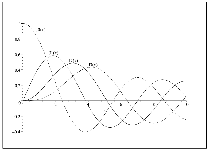
One solution of the differential equation is the Bessel function of the first kind of order \(p\), given as

\[y(x)=J_{p}(x)=\sum_{n=0}^{\infty} \dfrac{(-1)^{n}}{\Gamma(n+1) \Gamma(n+p+1)}\left(\dfrac{x}{2}\right)^{2 n+p} . \label{7.39} \]

In Figure 7.7 we display the first few Bessel functions of the first kind of integer order. Note that these functions can be described as decaying oscillatory functions.

Figure 7.7. Plots of the Bessel functions \(J_0(x), J_1(x), J_2(x)\), and \(J_3(x)\).

A second linearly independent solution is obtained for \(p\) not an integer as \(J_{-p}(x)\). However, for \(p\) an integer, the \(\Gamma(n+p+1)\) factor leads to evaluations of the Gamma function at zero, or negative integers, when \(p\) is negative. Thus, the above series is not defined in these cases.

Another method for obtaining a second linearly independent solution is through a linear combination of \(J_{p}(x)\) and \(J_{-p}(x)\) as

\[N_{p}(x)=Y_{p}(x)=\dfrac{\cos \pi p J_{p}(x)-J_{-p}(x)}{\sin \pi p} \label{7.40} \]

These functions are called the Neumann functions, or Bessel functions of the second kind of order \(p\).

In Figure 7.8 we display the first few Bessel functions of the second kind of integer order. Note that these functions are also decaying oscillatory functions. However, they are singular at \(x=0\).

In many applications these functions do not satisfy the boundary condition that one desires a bounded solution at \(x=0\). For example, one standard problem is to describe the oscillations of a circular drumhead. For this problem one solves the wave equation using separation of variables in cylindrical coordinates. The \(r\) equation leads to a Bessel equation. The Bessel function solutions describe the radial part of the solution and one does not expect a singular solution at the center of the drum. The amplitude of the oscillation must remain finite. Thus, only Bessel functions of the first kind can be used.

Bessel functions satisfy a variety of properties, which we will only list at this time for Bessel functions of the first kind.

Derivative Identities

\[\dfrac{d}{d x}\left[x^{p} J_{p}(x)\right]=x^{p} J_{p-1}(x) \label{7.41} \]

Figure 7.8. Plots of the Neumann functions \(N_{0}(x), N_{1}(x), N_{2}(x)\), and \(N_{3}(x)\).

\[\dfrac{d}{d x}\left[x^{-p} J_{p}(x)\right]=-x^{-p} J_{p+1}(x) \label{7.42} \]

Recursion Formulae

\[J_{p-1}(x)+J_{p+1}(x)=\dfrac{2 p}{x} J_{p}(x) \label{7.43} \]

\[J_{p-1}(x)-J_{p+1}(x)=2 J_{p}^{\prime}(x) \label{7.44} \]

Orthogonality

\[\int_{0}^{a} x J_{p}\left(j_{p n} \dfrac{x}{a}\right) J_{p}\left(j_{p m} \dfrac{x}{a}\right) d x=\dfrac{a^{2}}{2}\left[J_{p+1}\left(j_{p n}\right)\right]^{2} \delta_{n, m} \label{7.45} \]

where \(j_{p n}\) is the \(n\)th root of \(J_{p}(x), J_{p}\left(j_{p n}\right)=0, n=1,2, \ldots\) A list of some of these roots are provided in Table 7.4.

\(\begin{array}{c|c|c|c|c|c|c}
n & p=0 & p=1 & p=2 & p=3 & p=4 & p=5 \\
\hline 1 & 2.405 & 3.832 & 5.135 & 6.379 & 7.586 & 8.780 \\
2 & 5.520 & 7.016 & 8.147 & 9.760 & 11.064 & 12.339 \\
3 & 8.654 & 10.173 & 11.620 & 13.017 & 14.373 & 15.700 \\
4 & 11.792 & 13.323 & 14.796 & 16.224 & 17.616 & 18.982 \\
5 & 14.931 & 16.470 & 17.960 & 19.410 & 20.827 & 22.220 \\
6 & 18.071 & 19.616 & 21.117 & 22.583 & 24.018 & 25.431 \\
7 & 21.212 & 22.760 & 24.270 & 25.749 & 27.200 & 28.628 \\
8 & 24.353 & 25.903 & 27.421 & 28.909 & 30.371 & 31.813 \\
9 & 27.494 & 29.047 & 30.571 & 32.050 & 33.512 & 34.983
\end{array}\)

Table 7.4. The zeros of Bessel Functions

Generating Function

\[e^{x\left(t-\dfrac{1}{t}\right) / 2}=\sum_{n=-\infty}^{\infty} J_{n}(x) t^{n}, \quad x>0, t \neq 0 . \label{7.46} \]

Integral Representation

\[J_{n}(x)=\dfrac{1}{\pi} \int_{0}^{\pi} \cos (x \sin \theta-n \theta) d \theta, \quad x>0, n \in \mathrm{Z} . \label{7.47} \]

Fourier-Bessel Series

Since the Bessel functions are an orthogonal set of eigenfunctions of a Sturm-Liouville problem, we can expand square integrable functions in this basis. In fact, the eigenvalue problem is given in the form

\[x^{2} y^{\prime \prime}+x y^{\prime}+\left(\lambda x^{2}-p^{2}\right) y=0 . \label{7.48} \]

The solutions are then of the form \(J_{p}(\sqrt{\lambda} x)\), as can be shown by making the substitution \(t=\sqrt{\lambda} x\) in the differential equation.

Furthermore, one can solve the differential equation on a finite domain, \([0, a]\), with the boundary conditions: \(y(x)\) is bounded at \(x=0\) and \(y(a)= 0\). One can show that \(J_{p}\left(j_{p n} \dfrac{x}{a}\right)\) is a basis of eigenfunctions and the resulting Fourier-Bessel series expansion of \(f(x)\) defined on \(x \in[0, a]\) is

\[f(x)=\sum_{n=1}^{\infty} c_{n} J_{p}\left(j_{p n} \dfrac{x}{a}\right) \label{7.49} \]

where the Fourier-Bessel coefficients are found using the orthogonality relation as

\[c_{n}=\dfrac{2}{a^{2}\left[J_{p+1}\left(j_{p n}\right)\right]^{2}} \int_{0}^{a} x f(x) J_{p}\left(j_{p n} \dfrac{x}{a}\right) d x . \label{7.50} \]

Example 7.8. Expand \(f(x)=1\) for \(0 \leq x \leq 1\) in a Fourier-Bessel series of the form

\[f(x)=\sum_{n=1}^{\infty} c_{n} J_{0}\left(j_{0 n} x\right) \nonumber \]

We need only compute the Fourier-Bessel coefficients in Equation (7.50):

\[c_{n}=\dfrac{2}{\left[J_{1}\left(j_{0 n}\right)\right]^{2}} \int_{0}^{1} x J_{0}\left(j_{0 n} x\right) d x . \label{7.51} \]

From Equation (7.41) we have

\[\begin{aligned}
\int_{0}^{1} x J_{0}\left(j_{0 n} x\right) d x &=\dfrac{1}{j_{0 n}^{2}} \int_{0}^{j_{0 n}} y J_{0}(y) d y \\
&=\dfrac{1}{j_{0 n}^{2}} \int_{0}^{j_{0 n}} \dfrac{d}{d y}\left[y J_{1}(y)\right] d y \\
&=\dfrac{1}{j_{0 n}^{2}}\left[y J_{1}(y)\right]_{0}^{j_{0 n}} \\
&=\dfrac{1}{j_{0 n}} J_{1}\left(j_{0 n}\right)
\end{aligned} \label{7.52} \]

As a result, we have found that the desired Fourier-Bessel expansion is

\[1=2 \sum_{n=1}^{\infty} \dfrac{J_{0}\left(j_{0 n} x\right)}{j_{0 n} J_{1}\left(j_{0 n}\right)}, \quad 0<x<1 \label{7.53} \]

In Figure 7.9 we show the partial sum for the first fifty terms of this series. We see that there is slow convergence due to the Gibbs’ phenomenon. Note: For reference, the partial sums of the Fourier-Bessel series was computed in Maple using the following code:

2*sum(BesselJ(0,BesselJZeros(0,n)*x) 
/(BesselJZeros(0,n)*BesselJ(1,BesselJZeros(0,n))),n=1..50)

Figure 7.9. Plot of the first 50 terms of the Fourier-Bessel series in Equation (7.53) for \(f(x)=1\) on \(0<x<1\).