10.1: Distinct Real Eigenvalues

We illustrate the solution method by example.

Example: Find the general solution of \(\dot{x}_{1}=x_{1}+x_{2}, \dot{x}_{2}=4 x_{1}+x_{2}\).

View tutorial on YouTube

The equation to be solved may be rewritten in matrix form as

\[\frac{d}{d t}\left(\begin{array}{l} x_{1} \\ x_{2} \end{array}\right)=\left(\begin{array}{ll} 1 & 1 \\ 4 & 1 \end{array}\right)\left(\begin{array}{l} x_{1} \\ x_{2} \end{array}\right) \nonumber \]

or in short hand as Equation \ref{10.2}.

We take as our ansatz \(x(t)=v e^{\lambda t}\), where \(v\) and \(\lambda\) are independent of \(t\). Upon substitution into Equation \ref{10.2}, we obtain

\[\lambda \mathrm{v} e^{\lambda t}=\mathrm{Av}^{\lambda t} \nonumber \]

and upon cancellation of the exponential, we obtain the eigenvalue problem

\[\mathrm{Av}=\lambda \mathrm{v} . \nonumber \]

Finding the characteristic equation using Equation \ref{5.4}, we have

\[\begin{aligned} 0 &=\operatorname{det}(\mathrm{A}-\lambda \mathrm{I}) \\ &=\lambda^{2}-2 \lambda-3 \\ &=(\lambda-3)(\lambda+1) \end{aligned} \nonumber \]

Therefore, the two eigenvalues are \(\lambda_{1}=3\) and \(\lambda_{2}=-1\).

To determine the corresponding eigenvectors, we substitute the eigenvalues successively into

\[(\mathrm{A}-\lambda \mathrm{I}) \mathrm{v}=0 . \nonumber \]

We will write the corresponding eigenvectors \(v_{1}\) and \(v_{2}\) using the matrix notation

\[\left(\begin{array}{ll} \mathrm{v}_{1} & \mathrm{v}_{2} \end{array}\right)=\left(\begin{array}{ll} v_{11} & v_{12} \\ v_{21} & v_{22} \end{array}\right), \nonumber \]

where the components of \(v_{1}\) and \(v_{2}\) are written with subscripts corresponding to the first and second columns of a 2-by-2 matrix.

For \(\lambda_{1}=3\), and unknown eigenvector \(v_{1}\), we have from Equation \ref{10.5}

\[\begin{gathered} -2 v_{11}+v_{21}=0 \\ 4 v_{11}-2 v_{21}=0 \end{gathered} \nonumber \]

Clearly, the second equation is just the first equation multiplied by \(-2\), so only one equation is linearly independent. This will always be true, so for the 2 -by-2 case we need only consider the first row of the matrix. The first eigenvector therefore satisfies \(v_{21}=2 v_{11}\). Recall that an eigenvector is only unique up to multiplication by a constant: we may therefore take \(v_{11}=1\) for convenience.

For \(\lambda_{2}=-1\), and eigenvector \(v_{2}=\left(v_{12}, v_{22}\right)^{T}\), we have from Equation \ref{10.5}

\[2 v_{12}+v_{22}=0, \nonumber \]

so that \(v_{22}=-2 v_{12}\). Here, we take \(v_{12}=1\).

Therefore, our eigenvalues and eigenvectors are given by

\[\lambda_{1}=3, \mathrm{v}_{1}=\left(\begin{array}{l} 1 \\ 2 \end{array}\right) ; \quad \lambda_{2}=-1, \mathrm{v}_{2}=\left(\begin{array}{r} 1 \\ -2 \end{array}\right) \text {. } \nonumber \]

Using the principle of superposition, the general solution to the ode is therefore

\[X(t)=c_{1} v_{1} e^{\lambda_{1} t}+c_{2} v_{2} e^{\lambda_{2} t} \nonumber \]

or explicitly writing out the components,

\[\begin{aligned} &x_{1}(t)=c_{1} e^{3 t}+c_{2} e^{-t} \\ &x_{2}(t)=2 c_{1} e^{3 t}-2 c_{2} e^{-t} \end{aligned} \nonumber \]

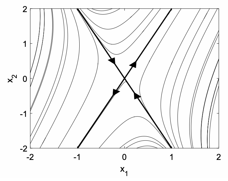
We can obtain a new perspective on the solution by drawing a phase portrait, shown in Fig. 10.1, with " \(\mathrm{x}\)-axis" \(x_{1}\) and " \(\mathrm{y}\)-axis" \(x_{2}\). Each curve corresponds to a different initial condition, and represents the trajectory of a particle with velocity given by the differential equation. The dark lines represent trajectories along the direction of the eigenvectors. If \(c_{2}=0\), the motion is along the eigenvector \(v_{1}\) with \(x_{2}=2 x_{1}\) and the motion with increasing time is away from the origin (arrows pointing out) since the eigenvalue \(\lambda_{1}=3>0\). If \(c_{1}=0\), the motion is along the eigenvector \(\mathrm{v}_{2}\) with \(x_{2}=-2 x_{1}\) and motion is towards the origin (arrows pointing in) since the eigenvalue \(\lambda_{2}=-1<0\). When the eigenvalues are real and of opposite signs, the origin is called a saddle point. Almost all trajectories (with the exception of those with initial conditions exactly satisfying \(x_{2}(0)=-2 x_{1}(0)\) ) eventually move away from the origin as \(t\) increases. When the eigenvalues are real and of the same sign, the origin is called a node. A node can be stable (negative eigenvalues) or unstable (positive eigenvalues).

Figure 10.1: Phase portrait for example with two real eigenvalues of opposite sign.