1.1: Integrals as solutions

A first order ODE is an equation of the form

$$\dfrac{dy}{dx}=f(x,y) \nonumber$$

or just

$$y'=f(x,y) \nonumber$$

In general, there is no simple formula or procedure one can follow to find solutions. In the next few lectures we will look at special cases where solutions are not difficult to obtain. In this section, let us assume that $f$ is a function of $x$ alone, that is, the equation is

$$y'=f(x) \label{1.1.1}$$

We could just integrate (antidifferentiate) both sides with respect to $x$.

$$\int y' (x) dx = \int f(x) dx + C \nonumber$$

that is

$$y(x)=\int f(x) dx + C \nonumber$$

This $y(x)$ is actually the general solution. So to solve Equation $\ref{1.1.1}$, we find some antiderivative of $f(x)$ and then we add an arbitrary constant to get the general solution.

Now is a good time to discuss a point about calculus notation and terminology. Calculus textbooks muddy the waters by talking about the integral as primarily the so-called indefinite integral. The indefinite integral is really the antiderivative (in fact the whole one-parameter family of antiderivatives). There really exists only one integral and that is the definite integral. The only reason for the indefinite integral notation is that we can always write an antiderivative as a (definite) integral. That is, by the fundamental theorem of calculus we can always write $\int f(x) dx + C$ as

$$\int_{x_0}^x f(t) dt + C \nonumber$$

Hence the terminology to integrate when we may really mean to antidifferentiate. Integration is just one way to compute the antiderivative (and it is a way that always works, see the following examples). Integration is defined as the area under the graph, it only happens to also compute antiderivatives. For sake of consistency, we will keep using the indefinite integral notation when we want an antiderivative, and you should always think of the definite integral.

Example $\PageIndex{1}$

Find the general solution of $y' = 3x^2$.

Solution

Elementary calculus tells us that the general solution must be $y = x^3 + C$. Let us check: $y' = 3x^2$. We have gotten precisely our equation back.

Normally, we also have an initial condition such as $y(x_0) = y_0$ for some two numbers${x_0}$ and ${y_0}$ ${x_0}$ is usually 0, but not always). We can then write the solution as a definite integral in a nice way. Suppose our problem is $y' = f(x), \, y(x_0) = y_0$. Then the solution is

$$y(x) = \int_{x_0}^x f(s) ds + y_0 \label{1.1.2}$$

Let us check! We compute $y' = f(x)$, via the fundamental theorem of calculus, and by Jupiter, $y$ is a solution. Is it the one satisfying the initial condition? Well, $y(x_0) = \int_{x_0}^{x_0} f(x) dx + y_0 = y_0$. It is!

Do note that the definite integral and the indefinite integral (antidifferentiation) are completely different beasts. The definite integral always evaluates to a number. Therefore, Equation $\ref{1.1.2}$ is a formula we can plug into the calculator or a computer, and it will be happy to calculate specific values for us. We will easily be able to plot the solution and work with it just like with any other function. It is not so crucial to always find a closed form for the antiderivative.

Example $\PageIndex{2}$

Solve

$$y' = e^{-x^2}, ~~ y(0) = 1. \nonumber$$

By the preceding discussion, the solution must be

$$y(x) = \int_0^x e^{-s^2} ds + 1. \nonumber$$

Solution

Here is a good way to make fun of your friends taking second semester calculus. Tell them to find the closed form solution. Ha ha ha (bad math joke). It is not possible (in closed form). There is absolutely nothing wrong with writing the solution as a definite integral. This particular integral is in fact very important in statistics.

Using this method, we can also solve equations of the form

$$y' = f(y) \nonumber$$

Let us write the equation in Leibniz notation.

$$\dfrac{dy}{dx} = f(y) \nonumber$$

Now we use the inverse function theorem from calculus to switch the roles of $x$ and $y$ to obtain

$$\dfrac{dy}{dx} = \dfrac{1}{f(y)} \nonumber$$

What we are doing seems like algebra with $dx$ and $dy$. It is tempting to just do algebra with $dx$ and $dy$ as if they were numbers. And in this case it does work. Be careful, however, as this sort of hand-waving calculation can lead to trouble, especially when more than one independent variable is involved. At this point we can simply integrate,

$$x(y) = \int \dfrac{1}{f(y)} dy + C \nonumber$$

Finally, we try to solve for $y$.

Example $\PageIndex{3}$

Previously, we guessed $y' = ky$ (for some $k > 0$) has the solution $y = Ce^{kx}$. We can now find the solution without guessing. First we note that $y = 0$ is a solution. Henceforth, we assume $y \ne 0$. We write

$$\dfrac{dx}{dy} = \dfrac{1}{ky} \nonumber$$

We integrate to obtain

$$x(y) = x = \dfrac{1}{k} \ln \left\vert y \right\vert + D \nonumber$$

where $D$ is an arbitrary constant. Now we solve for$y$ (actually for $\left\vert y \right\vert$ ).

$$\left\vert y \right\vert = e^{kx-kD} = e^{-kD}e^{kx} \nonumber$$

If we replace $e^{-kD}$ with an arbitrary constant $C$ we can get rid of the absolute value bars (which we can do as $D$ was arbitrary). In this way, we also incorporate the solution $y = 0$. We get the same general solution as we guessed before, $y = Ce^{kx}$.

Example $\PageIndex{4}$

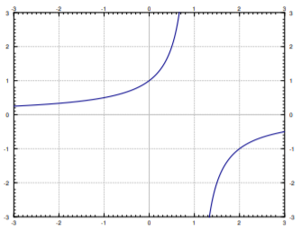
Find the general solution of $y' = y^2$.

Solution

First we note that $y = 0$ is a solution. We can now assume that $y \ne 0$. Write

$$\dfrac{dx}{dy} = \dfrac{1}{y^2} \nonumber$$

We integrate to get

$$x = \dfrac{-1}{y} + C \nonumber$$

We solve for $y = \dfrac{1}{C-x}$. So the general solution is

$$y = \dfrac{1}{C-x} \,\, or\,\, y=0 \nonumber$$

Note the singularities of the solution. If for example $C=1$, then the solution as we approach $x=1$. See Figure $\PageIndex{1}$. Generally, it is hard to tell from just looking at the equation itself how the solution is going to behave. The equation $y' = y^2$ is very nice and defined everywhere, but the solution is only defined on some interval $(-\infty, C)$ or $(C, \infty)$. Usually when this happens we only consider one of these the solution. For example if we impose a condition $y(0) = 1$, then the solution is $y=\frac{1}{1-x}$, and we would consider this solution only for $x$ on the interval $(-\infty,1)$. In the figure, it is the left side of the graph.

Figure $\PageIndex{1}$: Plot of $y=\frac{1}{1-x}$.

Classical problems leading to differential equations solvable by integration are problems dealing with velocity, acceleration and distance. You have surely seen these problems before in your calculus class.

Example $\PageIndex{5}$

Suppose a car drives at a speed $e^{t/2}$ meters per second, where $t$ is time in seconds. How far did the car get in 2 seconds (starting at $t = 0$)? How far in 10 seconds?

Solution

Let $x$ denote the distance the car traveled. The equation is

$$x' = e^{t/2} \nonumber$$

We can just integrate this equation to get that

$$x(t) = 2e^{t/2} + C \nonumber$$

We still need to figure out $C$. We know that when $t = 0$, then $x = 0$. That is, $x(0) = 0$. So

$$0 = x(0) = 2 e^{0/2} + C = 2 + C \nonumber$$

Thus $C = -2$ and

$$x(t) = 2 e^{t/2} - 2 \nonumber$$

Now we just plug in to get where the car is at 2 and at 10 seconds. We obtain

$$x(2) = 2e^{2/2} - 2 \approx 3.44 \text{~meters},~~~ x(10) = 2e^{10/2} - 2 \approx 294\text{~meters} \nonumber$$

Example $\PageIndex{6}$

Suppose that the car accelerates at a rate of $t^2 \frac{m}{s^2}$. At time $t = 0$ the car is at the 1 meter mark and is traveling at 10 ^m/_s. Where is the car at time $t = 10$.

Solution

Well this is actually a second order problem. If $x$ is the distance traveled, then $x'$ is the velocity, and $x''$ is the acceleration. The equation with initial conditions is

$$x'' = t^2, \quad x(0) = 1, \quad x'(0) = 10 \nonumber$$

What if we say $x' = v$. Then we have the problem

$$v' = t^2, \quad v(0) = 10 \nonumber$$

Once we solve for $v$, we can integrate and find $x$.