1.6: Autonomous equations
- Page ID
- 331
\( \newcommand{\vecs}[1]{\overset { \scriptstyle \rightharpoonup} {\mathbf{#1}} } \)
\( \newcommand{\vecd}[1]{\overset{-\!-\!\rightharpoonup}{\vphantom{a}\smash {#1}}} \)
\( \newcommand{\dsum}{\displaystyle\sum\limits} \)
\( \newcommand{\dint}{\displaystyle\int\limits} \)
\( \newcommand{\dlim}{\displaystyle\lim\limits} \)
\( \newcommand{\id}{\mathrm{id}}\) \( \newcommand{\Span}{\mathrm{span}}\)
( \newcommand{\kernel}{\mathrm{null}\,}\) \( \newcommand{\range}{\mathrm{range}\,}\)
\( \newcommand{\RealPart}{\mathrm{Re}}\) \( \newcommand{\ImaginaryPart}{\mathrm{Im}}\)
\( \newcommand{\Argument}{\mathrm{Arg}}\) \( \newcommand{\norm}[1]{\| #1 \|}\)
\( \newcommand{\inner}[2]{\langle #1, #2 \rangle}\)
\( \newcommand{\Span}{\mathrm{span}}\)
\( \newcommand{\id}{\mathrm{id}}\)
\( \newcommand{\Span}{\mathrm{span}}\)
\( \newcommand{\kernel}{\mathrm{null}\,}\)
\( \newcommand{\range}{\mathrm{range}\,}\)
\( \newcommand{\RealPart}{\mathrm{Re}}\)
\( \newcommand{\ImaginaryPart}{\mathrm{Im}}\)
\( \newcommand{\Argument}{\mathrm{Arg}}\)
\( \newcommand{\norm}[1]{\| #1 \|}\)
\( \newcommand{\inner}[2]{\langle #1, #2 \rangle}\)
\( \newcommand{\Span}{\mathrm{span}}\) \( \newcommand{\AA}{\unicode[.8,0]{x212B}}\)
\( \newcommand{\vectorA}[1]{\vec{#1}} % arrow\)
\( \newcommand{\vectorAt}[1]{\vec{\text{#1}}} % arrow\)
\( \newcommand{\vectorB}[1]{\overset { \scriptstyle \rightharpoonup} {\mathbf{#1}} } \)
\( \newcommand{\vectorC}[1]{\textbf{#1}} \)
\( \newcommand{\vectorD}[1]{\overrightarrow{#1}} \)
\( \newcommand{\vectorDt}[1]{\overrightarrow{\text{#1}}} \)
\( \newcommand{\vectE}[1]{\overset{-\!-\!\rightharpoonup}{\vphantom{a}\smash{\mathbf {#1}}}} \)
\( \newcommand{\vecs}[1]{\overset { \scriptstyle \rightharpoonup} {\mathbf{#1}} } \)
\(\newcommand{\longvect}{\overrightarrow}\)
\( \newcommand{\vecd}[1]{\overset{-\!-\!\rightharpoonup}{\vphantom{a}\smash {#1}}} \)
\(\newcommand{\avec}{\mathbf a}\) \(\newcommand{\bvec}{\mathbf b}\) \(\newcommand{\cvec}{\mathbf c}\) \(\newcommand{\dvec}{\mathbf d}\) \(\newcommand{\dtil}{\widetilde{\mathbf d}}\) \(\newcommand{\evec}{\mathbf e}\) \(\newcommand{\fvec}{\mathbf f}\) \(\newcommand{\nvec}{\mathbf n}\) \(\newcommand{\pvec}{\mathbf p}\) \(\newcommand{\qvec}{\mathbf q}\) \(\newcommand{\svec}{\mathbf s}\) \(\newcommand{\tvec}{\mathbf t}\) \(\newcommand{\uvec}{\mathbf u}\) \(\newcommand{\vvec}{\mathbf v}\) \(\newcommand{\wvec}{\mathbf w}\) \(\newcommand{\xvec}{\mathbf x}\) \(\newcommand{\yvec}{\mathbf y}\) \(\newcommand{\zvec}{\mathbf z}\) \(\newcommand{\rvec}{\mathbf r}\) \(\newcommand{\mvec}{\mathbf m}\) \(\newcommand{\zerovec}{\mathbf 0}\) \(\newcommand{\onevec}{\mathbf 1}\) \(\newcommand{\real}{\mathbb R}\) \(\newcommand{\twovec}[2]{\left[\begin{array}{r}#1 \\ #2 \end{array}\right]}\) \(\newcommand{\ctwovec}[2]{\left[\begin{array}{c}#1 \\ #2 \end{array}\right]}\) \(\newcommand{\threevec}[3]{\left[\begin{array}{r}#1 \\ #2 \\ #3 \end{array}\right]}\) \(\newcommand{\cthreevec}[3]{\left[\begin{array}{c}#1 \\ #2 \\ #3 \end{array}\right]}\) \(\newcommand{\fourvec}[4]{\left[\begin{array}{r}#1 \\ #2 \\ #3 \\ #4 \end{array}\right]}\) \(\newcommand{\cfourvec}[4]{\left[\begin{array}{c}#1 \\ #2 \\ #3 \\ #4 \end{array}\right]}\) \(\newcommand{\fivevec}[5]{\left[\begin{array}{r}#1 \\ #2 \\ #3 \\ #4 \\ #5 \\ \end{array}\right]}\) \(\newcommand{\cfivevec}[5]{\left[\begin{array}{c}#1 \\ #2 \\ #3 \\ #4 \\ #5 \\ \end{array}\right]}\) \(\newcommand{\mattwo}[4]{\left[\begin{array}{rr}#1 \amp #2 \\ #3 \amp #4 \\ \end{array}\right]}\) \(\newcommand{\laspan}[1]{\text{Span}\{#1\}}\) \(\newcommand{\bcal}{\cal B}\) \(\newcommand{\ccal}{\cal C}\) \(\newcommand{\scal}{\cal S}\) \(\newcommand{\wcal}{\cal W}\) \(\newcommand{\ecal}{\cal E}\) \(\newcommand{\coords}[2]{\left\{#1\right\}_{#2}}\) \(\newcommand{\gray}[1]{\color{gray}{#1}}\) \(\newcommand{\lgray}[1]{\color{lightgray}{#1}}\) \(\newcommand{\rank}{\operatorname{rank}}\) \(\newcommand{\row}{\text{Row}}\) \(\newcommand{\col}{\text{Col}}\) \(\renewcommand{\row}{\text{Row}}\) \(\newcommand{\nul}{\text{Nul}}\) \(\newcommand{\var}{\text{Var}}\) \(\newcommand{\corr}{\text{corr}}\) \(\newcommand{\len}[1]{\left|#1\right|}\) \(\newcommand{\bbar}{\overline{\bvec}}\) \(\newcommand{\bhat}{\widehat{\bvec}}\) \(\newcommand{\bperp}{\bvec^\perp}\) \(\newcommand{\xhat}{\widehat{\xvec}}\) \(\newcommand{\vhat}{\widehat{\vvec}}\) \(\newcommand{\uhat}{\widehat{\uvec}}\) \(\newcommand{\what}{\widehat{\wvec}}\) \(\newcommand{\Sighat}{\widehat{\Sigma}}\) \(\newcommand{\lt}{<}\) \(\newcommand{\gt}{>}\) \(\newcommand{\amp}{&}\) \(\definecolor{fillinmathshade}{gray}{0.9}\)Let us consider general differential equation problems of the form
\[ \dfrac{dx}{dt} = f(x) \nonumber \]
where the derivative of solutions depends only on \(x\) (the dependent variable). Such equations are called autonomous equations. If we think of \(t\) as time, the naming comes from the fact that the equation is independent of time.
Let us come back to the cooling coffee problem (see Example 1.3.3). Newton’s law of cooling says that
\[ \dfrac{dx}{dt} = -k(x-A) \nonumber \]
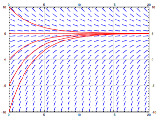
where \(x\) is the temperature, \(t\) is time, \(k\) is some constant, and \(A\) is the ambient temperature. See Figure \(\PageIndex{1}\) for an example with \(k = 0.3\) and \(A = 5\).
Note the solution \(x = A\) (in the figure \(x = 5\)). We call these constant solutions the equilibrium solutions. The points on the \(x\) axis where \(f(X) = 0\) are called critical points. The point \(x = A\) is a critical point. In fact, each critical point corresponds to an equilibrium solution. Note also, by looking at the graph, that the solution \(x = A\) is “stable” in that small perturbations in \(x\) do not lead to substantially different solutions as \(t\) grows. If we change the initial condition a little bit, then as \(t \rightarrow \infty \) we get \(x \rightarrow A\). We call such critical points stable. In this simple example it turns out that all solutions in fact go to \(A\) as \( t \rightarrow \infty\). If a critical point is not stable we would say it is unstable.
Let us consider the logistic equation
\[ \dfrac{dx}{dt} = kx(M-x) \nonumber \]
for some positive \(k\) and \(M\). This equation is commonly used to model population if we know the limiting population \(M\), that is the maximum sustainable population. The logistic equation leads to less catastrophic predictions on world population than \(x'=kx\). In the real world there is no such thing as negative population, but we will still consider negative \(x\) for the purposes of the math (see Figure \(\PageIndex{2}\) for an example).
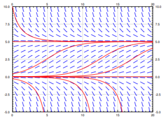
Note two critical points, \(x = 0\) and \(x = 5\). The critical point at \(x = 5\). is stable. On the other hand the critical point at \(x = 0\). is unstable.
It is not really necessary to find the exact solutions to talk about the long term behavior of the solutions. For example, from the above slope field plot, we can easily see that
\[\lim\limits_{t\to\infty} x(t) = \begin{cases} 5 & \text{if} \, x(0) > 0, \\ 0 & \text{if} \, x(0) = 0, \\ \text{DNE or} -\infty & \text{if} \, x(0) < 0. \end{cases} \nonumber \]
Where DNE means “does not exist.” From just looking at the slope field we cannot quite decide what happens if \(x(0) < 0\). It could be that the solution does not exist for \(t\) all the way to \(\infty\). Think of the equation \(x' = x^2\), we have seen that it only exists for some finite period of time. Same can happen here. In our example equation above it will actually turn out that the solution does not exist for all time, but to see that we would have to solve the equation. In any case, the solution does go to \(- \infty\), but it may get there rather quickly.
If we are interested only in the long term behavior of the solution, we would be doing unnecessary work if we solved the equation exactly. We could draw the slope field, but it is easier to just look at the or , which is a simple way to visualize the behavior of autonomous equations. In this case there is one dependent variable \(x\). We draw the \(x\)-axis, we mark all the critical points, and then we draw arrows in between. Since \(x\) is the dependent variable we draw the axis vertically, as it appears in the slope field diagrams above. If \(f(x) > 0\), we draw an up arrow. If \(f(x) < 0\), we draw a down arrow. To figure this out, we could just plug in some \(x\) between the critical points, \(f(x)\) will have the same sign at all \(x\) between two critical points as long \(f(x)\) is continuous. For example, \(f(6) = -0.6 < 0\), so \(f(x) < 0\) for \(x > 5\), and the arrow above \(x=5\) is a down arrow. Next, \(f(1) = 0.4 > 0\), so \(f(x) > 0\) whenever \(0 < x < 5\), and the arrow points up. Finally, \(f(-1) = -0.6 < 0\) so \(f(x) < 0\) when \(x < 0\), and the arrow points down.

Armed with the phase diagram, it is easy to sketch the solutions approximately: As time \(t\) moves from left to right, the graph of a solution goes up if the arrow is up, and it goes down if the arrow is down.
Try sketching a few solutions simply from looking at the phase diagram. Check with the preceding graphs if you are getting the type of curves.
Once we draw the phase diagram, we can easily classify critical points as stable or unstable.\(^{1}\)

Since any mathematical model we cook up will only be an approximation to the real world, unstable points are generally bad news.
Let us think about the logistic equation with harvesting. Suppose an alien race really likes to eat humans. They keep a planet with humans on it and harvest the humans at a rate of \(h\) million humans per year. Suppose\(x\) is the number of humans in millions on the planet and \(t\) is time in years. Let \(M\) be the limiting population when no harvesting is done and \(k>0\) is some constant depending on how fast humans multiply. Our equation becomes
\[ \dfrac{dx}{dt} = kx(M-x)-h \nonumber \]
We expand the right hand side and solve for critical points
\[ \dfrac{dx}{dt} = -kx^2+kMx-h \nonumber \]
Solving for the critical points \( A\) and \(B\) from the quadratic equations:
\[ A= \dfrac{kM + \sqrt{(kM)^2-4hk}}{2k},\quad B= \dfrac{kM - \sqrt{(kM)^2-4hk}}{2k} \nonumber \]
Sketch a phase diagram for different possibilities. Note that these possibilities are \(A > B\), or \(A = B\), or \(A\) and \(B\) both complex (i.e. no real solutions). Hint: Fix some simple \(k\) and \(M\) and then vary \(h\).
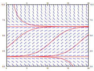
For example, let \(M=8\) and \(k=0.1\). When \(h=1\), then \(A\) and \(B\) are distinct and positive. The slope field we get is in Figure \(\PageIndex{5}\). As long as the population starts above \(B\), which is approximately 1.55 million, then the population will not die out. It will in fact tend towards \(A \approx 6.45\) million. If ever some catastrophe happens and the population drops below \(B\), humans will die out, and the fast food restaurant serving them will go out of business.
When \(h=1.6\), then \(A=B=4\) and there is only one critical point and it is unstable. When the population starts above 4 million it will tend towards 4 million. If it ever drops below 4 million, humans will die out on the planet. This scenario is not one that we (as the human fast food proprietor) want to be in. A small perturbation of the equilibrium state and we are out of business; there is no room for error (see Figure \(\PageIndex{6}\)).
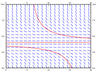
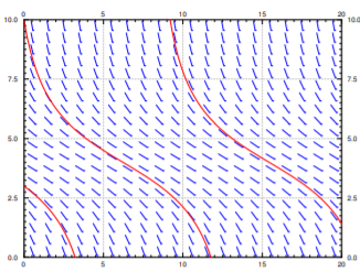
Finally if we are harvesting at 2 million humans per year, there are no critical points. The population will always plummet towards zero, no matter how well stocked the planet starts (see Figure \(\PageIndex{7}\)).
Footnotes
[1] Unstable points with one of the arrows pointing towards the critical point are sometimes called semistable.
References
- Paul W. Berg and James L. McGregor, Elementary Partial Differential Equations, Holden-Day, San Francisco, CA, 1966.
- William E. Boyce, Richard C. DiPrima, Elementary Differential Equations and Boundary Value Problems, 9th edition, John Wiley & Sons Inc., New York, NY, 2008.
- C.H. Edwards and D.E. Penney, Differential Equations and Boundary Value Problems: Computing and Modeling, 4th edition, Prentice Hall, 2008.
- Stanley J. Farlow, An Introduction to Differential Equations and Their Applications, McGraw-Hill, Inc., Princeton, NJ, 1994. (Published also by Dover Publications, 2006.)
- E.L. Ince, Ordinary Differential Equations, Dover Publications, Inc., New York, NY, 1956.


