3: Behavior Near Trajectories and Invariant Sets - Stability

Consider the general nonautonomous vector field in n dimensions:

$$\begin{array}{}\text{(3.1)}& \dot{x}=f(x,t),x\in {\mathbb{R}}^n,\end{array}$$

and let $\overline{x}(t,t_0,x_0)$ be a solution of this vector field.

Many questions in ODEs concern understanding the behavior of neighboring solutions near a given, chosen solution. We will develop the general framework for considering such questions by transforming Equation $\text{3.1}$ to a form that allows us to explicitly consider these issues.

We consider the following (time dependent) transformation of variables:

$$\begin{array}{}\text{(3.2)}& x=y+\overline{x}(t,t_0,x_0).\end{array}$$

We wish to express Equation $\text{3.1}$ in terms of the y variables. It is important to understand what this will mean in terms of Equation $\text{3.2}$. For y small it means that x is near the solution of interest, $\overline{x}(t,t_0,x_0)$. In other words, expressing the vector field in terms of y will provide us with an explicit form of the vector field for studying the behavior near $\overline{x}(t,t_0,x_0)$. Towards this end, we begin by transforming Equation $\text{3.1}$ using Equation $\text{3.2}$ as follows:

$$\begin{array}{}\text{(3.3)}& \dot{x}=\dot{y}+\dot{\overline{x}}=f(x,t)=f(y+\overline{x},t),\end{array}$$

or

$\dot{y}=f(y+\overline{x},t)-\dot{\overline{x}}$,

$$\begin{array}{}\text{(3.4)}& =f(y+\overline{x},t)-f(\overline{x},t)\equiv g(y,t),g(0,t)=0.\end{array}$$

Hence, we have shown that solutions of Equation $\text{3.1}$ near $\overline{x}(t,t_0,x_0)$ are equivalent to solutions of Equation $\text{3.4}$ near y = 0.

The first question we want to ask related to the behavior near $\overline{x}(t,t_0,x_0)$ is whether or not this solution is stable? However, first we need to mathematically define what is meant by this term ''stable''. Now we should know that, without loss of generality, we can discuss this question in terms of the zero solution of Equation $\text{3.4}$.

We begin by defining the notion of ''Lyapunov stability'' (or just "stability").

We have several comments about these Definitions.

• Roughly speaking, a Lyapunov stable solution means that if you start close to that solution, you stay close–forever. Asymptotic stability not only means that you start close and stay close forever, but that you actually get "closer and closer" to the solution.
• Stability is an infinite time concept.
• If the ODE is autonomous, then the quantity $\delta =\delta (t_0,ϵ)$ can be chosen to be independent of $t_0$.
• The Definitions of stability do not tell us how to prove that a solution is stable (or unstable). We will learn two techniques for analyzing this question–linearization and Lyapunov’s (second) method.
• Why is Lyapunov stability included in the Definition of asymptotic stability? Because it is possible to construct examples where nearby solutions do get closer and closer to the given solution as $t\to \mathrm{\infty }$, but in the process there are intermediate intervals of time where nearby solutions make "large excursions" away from the given solution.

"Stability" is a notion that applies to a "neighborhood" of a trajectory. At this point we want to formalize various notions related to distance and neighborhoods in phase space. For simplicity in expressing these ideas we will take as our phase space Rn. Points in this phase space are denoted $x\in {\mathbb{R}}^n$, $x\equiv (x_1,...,x_n)$. The norm, or length, of x, denoted |x| is defined as:

$$\begin{array}{}\text{(3.7)}& |x|=\sqrt{x_1^2+x_2^2+\cdots +x_n^2}=\sqrt{\sum _{i=1}^n{x}_i^2}.\end{array}$$

The distance between two points in $x,y\in {\mathbb{R}}^n$ is defined as:

$$\begin{array}{}\text{(3.8)}& d(x,y)\equiv |x-y|=\sqrt{{(x_1-y_1)}^2+\cdots +{(x_n-y_n)}^2}\end{array}$$

\[= \sqrt{\sum_{i=1}^{n} \sqrt{(x_{i}-y_{i})^2}. \label{3.7}\]

Distance between points in ${\mathbb{R}}^n$ should be somewhat familiar, but now we introduce a new concept, the distance between a point and a set. Consider a set M, $M\subset {\mathbb{R}}^n$, let $p\in {\mathbb{R}}^n$. Then the distance from p to M is defined as follows:

$$\begin{array}{}\text{(3.9)}& dist(p,M)\equiv in{f}_{x\in M}|p-x|.\end{array}$$

We remark that it follows from the Definition that if $p\in M$, then dist(p, M) = 0.

We have previously defined the notion of an invariant set. Roughly speaking, invariant sets are comprised of trajectories. We now have the background to discuss the notion of . Recall, that the notion of invariant set was only developed for autonomous vector fields. So we consider an autonomous vector field:

$$\begin{array}{}\text{(3.10)}& \dot{x}=f(x),x\in {\mathbb{R}}^n,\end{array}$$

and denote the flow generated by this vector field by ${\varphi }_t(\cdot )$. Let M be a closed invariant set (in many applications we may also require M to be bounded) and let U M denoted a neighborhood of M.

The definition of Lyapunov stability of an invariant set is as follows.

In the dynamical systems approach to ordinary differential equations some alternative terminology is typically used.

The significance of attracting sets is that they are the "observable" regions in phase space since they are regions to which trajectories evolve in time. The set of points that evolve towards a specific attracting set is referred to as the basin of attraction for that invariant set.

We now consider an example that allows us to explicitly explore these ideas.

Example $3.9$

Consider the following autonomous vector field on the plane:

$\dot{x}=x$,

$$\begin{array}{}\text{(3.11)}& \dot{y}=y^2(1-y^2)\equiv f(y),(x,y)\in {\mathbb{R}}^2.\end{array}$$

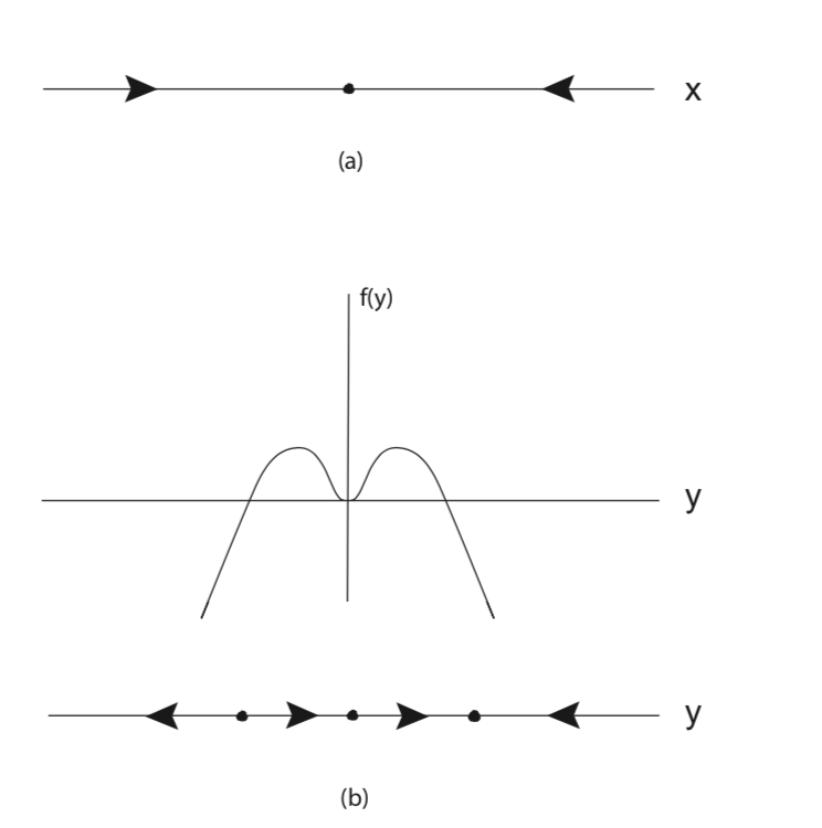
First, it is useful to note that the x and y components of Equation $\text{3.11}$ are independent. Consequently, this may seem like a trivial example. However, we will see that such examples provide a great deal of insight, especially since they allow for simple computations of many of the mathematical ideas.

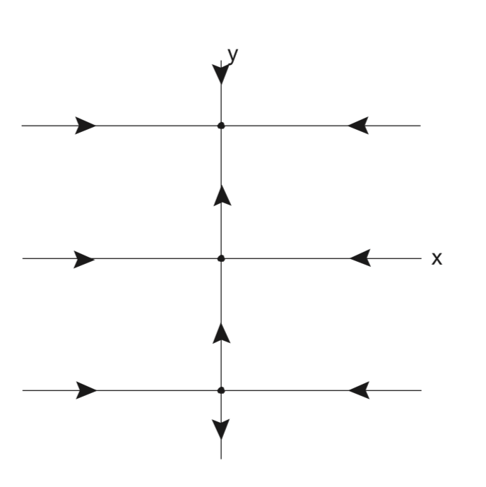
In Fig. 3.1 we illustrate the flow of the x and y components of Equation $\text{3.11}$ separately.

The two dimensional vector field Equation $\text{3.11}$ has equilibrium points at: (x, y) = (0, 0), (0, 1), $(0,-1)$.

In this example it is easy to identify three invariant horizontal lines (examples of invariant sets). Since y = 0 implies that $\dot{y}=0$, this implies that the x axis is invariant. Since y = 1 implies that $\dot{y}=0$, this implies that the line y = 1 is invariant. Since $y=-1$ implies that $\dot{y}=0$, which implies that the line $y=-1$ is invariant. This is illustrated in Fig. 3.2. Below we provide some additional invariant sets for (3.10). It is instructive to understand why they are invariant, and whether or not there are other invariant sets.

Additional invariant sets for (3.10).

{(x, y)| },

{(x, y)| },

{(x, y)| },

{(x, y)| },

{(x, y)| },

{(x, y)| },

{(x, y)| },

{(x, y)| }.

​​​​​​