
2: Special Structure and Solutions of ODEs
- Page ID
- 24137

\( \newcommand{\vecs}[1]{\overset { \scriptstyle \rightharpoonup} {\mathbf{#1}} } \)
\( \newcommand{\vecd}[1]{\overset{-\!-\!\rightharpoonup}{\vphantom{a}\smash {#1}}} \)
\( \newcommand{\dsum}{\displaystyle\sum\limits} \)
\( \newcommand{\dint}{\displaystyle\int\limits} \)
\( \newcommand{\dlim}{\displaystyle\lim\limits} \)
\( \newcommand{\id}{\mathrm{id}}\) \( \newcommand{\Span}{\mathrm{span}}\)
( \newcommand{\kernel}{\mathrm{null}\,}\) \( \newcommand{\range}{\mathrm{range}\,}\)
\( \newcommand{\RealPart}{\mathrm{Re}}\) \( \newcommand{\ImaginaryPart}{\mathrm{Im}}\)
\( \newcommand{\Argument}{\mathrm{Arg}}\) \( \newcommand{\norm}[1]{\| #1 \|}\)
\( \newcommand{\inner}[2]{\langle #1, #2 \rangle}\)
\( \newcommand{\Span}{\mathrm{span}}\)
\( \newcommand{\id}{\mathrm{id}}\)
\( \newcommand{\Span}{\mathrm{span}}\)
\( \newcommand{\kernel}{\mathrm{null}\,}\)
\( \newcommand{\range}{\mathrm{range}\,}\)
\( \newcommand{\RealPart}{\mathrm{Re}}\)
\( \newcommand{\ImaginaryPart}{\mathrm{Im}}\)
\( \newcommand{\Argument}{\mathrm{Arg}}\)
\( \newcommand{\norm}[1]{\| #1 \|}\)
\( \newcommand{\inner}[2]{\langle #1, #2 \rangle}\)
\( \newcommand{\Span}{\mathrm{span}}\) \( \newcommand{\AA}{\unicode[.8,0]{x212B}}\)
\( \newcommand{\vectorA}[1]{\vec{#1}} % arrow\)
\( \newcommand{\vectorAt}[1]{\vec{\text{#1}}} % arrow\)
\( \newcommand{\vectorB}[1]{\overset { \scriptstyle \rightharpoonup} {\mathbf{#1}} } \)
\( \newcommand{\vectorC}[1]{\textbf{#1}} \)
\( \newcommand{\vectorD}[1]{\overrightarrow{#1}} \)
\( \newcommand{\vectorDt}[1]{\overrightarrow{\text{#1}}} \)
\( \newcommand{\vectE}[1]{\overset{-\!-\!\rightharpoonup}{\vphantom{a}\smash{\mathbf {#1}}}} \)
\( \newcommand{\vecs}[1]{\overset { \scriptstyle \rightharpoonup} {\mathbf{#1}} } \)
\(\newcommand{\longvect}{\overrightarrow}\)
\( \newcommand{\vecd}[1]{\overset{-\!-\!\rightharpoonup}{\vphantom{a}\smash {#1}}} \)
\(\newcommand{\avec}{\mathbf a}\) \(\newcommand{\bvec}{\mathbf b}\) \(\newcommand{\cvec}{\mathbf c}\) \(\newcommand{\dvec}{\mathbf d}\) \(\newcommand{\dtil}{\widetilde{\mathbf d}}\) \(\newcommand{\evec}{\mathbf e}\) \(\newcommand{\fvec}{\mathbf f}\) \(\newcommand{\nvec}{\mathbf n}\) \(\newcommand{\pvec}{\mathbf p}\) \(\newcommand{\qvec}{\mathbf q}\) \(\newcommand{\svec}{\mathbf s}\) \(\newcommand{\tvec}{\mathbf t}\) \(\newcommand{\uvec}{\mathbf u}\) \(\newcommand{\vvec}{\mathbf v}\) \(\newcommand{\wvec}{\mathbf w}\) \(\newcommand{\xvec}{\mathbf x}\) \(\newcommand{\yvec}{\mathbf y}\) \(\newcommand{\zvec}{\mathbf z}\) \(\newcommand{\rvec}{\mathbf r}\) \(\newcommand{\mvec}{\mathbf m}\) \(\newcommand{\zerovec}{\mathbf 0}\) \(\newcommand{\onevec}{\mathbf 1}\) \(\newcommand{\real}{\mathbb R}\) \(\newcommand{\twovec}[2]{\left[\begin{array}{r}#1 \\ #2 \end{array}\right]}\) \(\newcommand{\ctwovec}[2]{\left[\begin{array}{c}#1 \\ #2 \end{array}\right]}\) \(\newcommand{\threevec}[3]{\left[\begin{array}{r}#1 \\ #2 \\ #3 \end{array}\right]}\) \(\newcommand{\cthreevec}[3]{\left[\begin{array}{c}#1 \\ #2 \\ #3 \end{array}\right]}\) \(\newcommand{\fourvec}[4]{\left[\begin{array}{r}#1 \\ #2 \\ #3 \\ #4 \end{array}\right]}\) \(\newcommand{\cfourvec}[4]{\left[\begin{array}{c}#1 \\ #2 \\ #3 \\ #4 \end{array}\right]}\) \(\newcommand{\fivevec}[5]{\left[\begin{array}{r}#1 \\ #2 \\ #3 \\ #4 \\ #5 \\ \end{array}\right]}\) \(\newcommand{\cfivevec}[5]{\left[\begin{array}{c}#1 \\ #2 \\ #3 \\ #4 \\ #5 \\ \end{array}\right]}\) \(\newcommand{\mattwo}[4]{\left[\begin{array}{rr}#1 \amp #2 \\ #3 \amp #4 \\ \end{array}\right]}\) \(\newcommand{\laspan}[1]{\text{Span}\{#1\}}\) \(\newcommand{\bcal}{\cal B}\) \(\newcommand{\ccal}{\cal C}\) \(\newcommand{\scal}{\cal S}\) \(\newcommand{\wcal}{\cal W}\) \(\newcommand{\ecal}{\cal E}\) \(\newcommand{\coords}[2]{\left\{#1\right\}_{#2}}\) \(\newcommand{\gray}[1]{\color{gray}{#1}}\) \(\newcommand{\lgray}[1]{\color{lightgray}{#1}}\) \(\newcommand{\rank}{\operatorname{rank}}\) \(\newcommand{\row}{\text{Row}}\) \(\newcommand{\col}{\text{Col}}\) \(\renewcommand{\row}{\text{Row}}\) \(\newcommand{\nul}{\text{Nul}}\) \(\newcommand{\var}{\text{Var}}\) \(\newcommand{\corr}{\text{corr}}\) \(\newcommand{\len}[1]{\left|#1\right|}\) \(\newcommand{\bbar}{\overline{\bvec}}\) \(\newcommand{\bhat}{\widehat{\bvec}}\) \(\newcommand{\bperp}{\bvec^\perp}\) \(\newcommand{\xhat}{\widehat{\xvec}}\) \(\newcommand{\vhat}{\widehat{\vvec}}\) \(\newcommand{\uhat}{\widehat{\uvec}}\) \(\newcommand{\what}{\widehat{\wvec}}\) \(\newcommand{\Sighat}{\widehat{\Sigma}}\) \(\newcommand{\lt}{<}\) \(\newcommand{\gt}{>}\) \(\newcommand{\amp}{&}\) \(\definecolor{fillinmathshade}{gray}{0.9}\)A consistent theme throughout all of ODEs is that ''special structure'' of the equations can reveal insight into the nature of the solutions. Here we look at a very basic and important property of autonomous equations:
"Time shifts of solutions of autonomous ODEs are also solutions of the ODE (but with a different initial condition)".
Now we will show how to see this.
Throughout this course we will assume that existence and uniqueness of solutions holds on a domain and time interval sufficient for our arguments and calculations.
We start by establishing the setting. We consider an autonomous vector field defined on \(\mathbb{R}^n\):
\[\dot{x} = f(x) \quad x(0) = x_{0}, \quad x \in \mathbb{R}^n, \label{2.1}\]
with solution denoted by:
\[x(t, 0, x_{0}), \,x(0, 0, x_{0}) = x_{0}.\]
Here we are taking the initial time to be \(t_{0} = 0\). We will see, shortly, that for autonomous equations this can be done without loss of generality. Now we choose \(s \in \mathbb{R}\) (\(s \ne 0\), which is to be regarded as a fixed constant). We must show the following:
\[\dot{x}(t+s) = f(x(t+s))\label{2.2}\]
This is what we mean by the phrase time shifts of solutions are solutions. This relation follows immediately from the chain rule calculation:
\[\frac{d}{dt} = \frac{d}{d(t+s)} \frac{d(t+s)}{dt} = \frac{d}{d(t+s)}. \label{2.3}\]
Finally, we need to determine the initial condition for the time shifted solution. For the original solution we have:
\[x(t, 0, x_{0}), x(0, 0, x_{0}) = x_{0}, \label{2.4}\]
and for the time shifted solution we have:
\[x(t + s, 0, x_{0}), x(s, 0, x_{0}). \label{2.5}\]
It is for this reason that, without loss of generality, for autonomous vector fields we can take the initial time to be \(t_{0} = 0\). This allows us to simplify the arguments in the notation for solutions of autonomous vector fields, i.e., \(x(t, 0, x_{0}) \equiv x(t, x_{0})\) with \(x(0, 0, x_{0}) = x(0, x_{0}) = x_{0}\).
Example \(\PageIndex{5}\): The time-shift property of autonomous vector fields
Consider the following one dimensional autonomous vector field:
\[\dot{x} = \lambda x, x(0) = x_{0}, x \in \mathbb{R}, \lambda \in \mathbb{R}. \nonumber\]
The solution is given by:
\[x(t, 0, x_{0}) = x(t, x_{0}) = e^{\lambda t}x_{0}. \nonumber\]
The time shifted solution is given by:
\[x(t+s, x_{0}) = e^{\lambda (t+s)}x_{0}. \nonumber\]
We see that it is a solution of the ODE with the following calculations:
\[\frac{d}{dt}x(t+s, x_{0}) = \lambda e^{\lambda (t+s)}x_{0} = \lambda x(t+s, x_{0}), \nonumber\]
with initial condition:
\[x(s, x_{0}) = e^{\lambda s}x_{0}. \nonumber\]
In summary, we see that the solutions of autonomous vector fields satisfy the following three properties:
- \(x(0, x_{0}) = x_{0}\)
- \(x(t, x_{0})\) is \(C^{r}\) in \(x_{0}\)
- \(x(t+s, x_{0}) = x(t, x(s, x_{0}))\)
Property one just reflects the notation we have adopted. Property 2 is a statement of the properties arising from existence and uniqueness of solutions. Property 3 uses two characteristics of solutions. One is the ''time shift'' property for autonomous vector fields that we have proven. The other is ''uniqueness of solutions'' since the left hand side and the right hand side of Property 3 satisfy the same initial condition at t = 0.
These three properties are the defining properties of a flow, i.e., a . In other words, we view the solutions as defining a map of points in phase space. The group property arises from property 3, i.e., the time-shift property. In order to emphasize this ''map of phase space'' property we introduce a general notation for the flow as follows
\[x(t, x_{0}) \equiv \phi_{t}(\cdot) \nonumber\]
where the ''·'' in the argument of \(\phi_{t}(\cdot)\) reflects the fact that the flow is a function on the phase space. With this notation the three properties of a flow are written as follows:
- \(\phi_{0}(\cdot)\) is the identity map.
- \(\phi_{t}(\cdot)\) is \(C^r\) for each t.
- \(\phi_{t+s}(\cdot) = \phi_{t} \circ \phi_{s}(\cdot)\)
We often use the phrase ''the flow generated by the (autonomous) vector field''. Autonomous is in parentheses as it is understood that when we are considering flows then we are considering the solutions of autonomous vector fields. This is because nonautonomous vector fields do not necessarily satisfy the time-shift property, as we now show with an example.
Example \(\PageIndex{6}\): An example of a nonautonomous vector field not having the time-shift property
Consider the following one dimensional vector field on \(\mathbb{R}\):
\[\dot{x} = \lambda tx\), \)x(0) = x_{0}, x \in \mathbb{R}\), \(\lambda \in \mathbb{R}. \nonumber\]
This vector field is separable and the solution is easily found to be:
\[x(t, 0, x_{0}) = x_{0}e^{\frac{\lambda}{2}t^2}. \nonumber\]
The time shifted ‘’solution” is given by:
\[x(t+s, 0, x_{0}) = x_{0}e^{\frac{\lambda}{2}(t+s)^2}. \nonumber \]
We show that this does not satisfy the vector field with the following calculation:
\(\frac{d}{dt}x(t+s, 0, x_{0}) = x_{0}e^{\frac{\lambda}{2}(t+s)^2}\lambda (t+s)\).
\(\ne \lambda tx(t+s, 0, x_{0})\).
Perhaps a more simple example illustrating that nonautonomous vector fields do not satisfy the time-shift property is the following.
Example \(\PageIndex{7}\)
Consider the following one dimensional nonautonomous vector field:
\(\dot{x} = e^{t}\), \(x \in \mathbb{R}\).
The solution is given by:
\(x(t) = e^t\).
It is easy to verify that the time-shifted function:
\(x(t+s) = e^{t+s}\),
does not satisfy the equation.
In the study of ODEs certain types of solutions have achieved a level of prominence largely based on their significance in applications. They are
- equilibrium solutions,
- periodic solutions,
- heteroclinic solutions,
- homoclinic solutions.
We define each of these.
DEFINITION 8: EQUILIBRIUM
A point in phase space \(x = \bar{x} = \mathbb{R}^n\) that is a solution of the ODE , i.e.
\(f(\bar{x}) = 0, f(\bar{x}, t) = 0\),
is called an equilibrium point.
For example, x = 0 is an equilibrium point for the following autonomous and nonautonomous one dimensional vector fields, respectively,
- \(\dot{x} = x\), \(x \in \mathbb{R}\),
- \(\dot{x} = tx\), \(x \in \mathbb{R}\).
A periodic solution is simply a solution that is periodic in time. Its definition is the same for both autonomous and nonautonomous vector fields.
DEFINITION 9: PERIODIC SolutionS
A solution \(x(t, t_{0}, x_{0})\) is periodic if there exists a T > 0 such that
\(x(t, t_{0}, x_{0}) = x(t+T, t_{0}, x_{0})\)
Homoclinic and heteroclinic solutions are important in a variety of applications. Their definition is not so simple as the definitions of equilibrium and periodic solutions since they can be defined and generalized to many different settings. We will only consider these special solutions for autonomous vector fields, and solutions homoclinic or heteroclinic to equilibrium solutions.
DEFINITION 10 (HOMOCLINIC AND HETEROCLINIC SolutionS)
Suppose \(\bar{x}_{1}\) and \(\bar{x}_{2}\) are equilibrium points of an autonomous vector field, i.e.
\(f(\bar{x}_{1}) = 0\), \(f(\bar{x}_{2}) = 0\).
A trajectory \(x(t, t_{0}, x_{0})\) is said to be heteroclinic to \(\bar{x}_{1}\) and \(\bar{x}_{2}\) if
\(lim_{t \rightarrow \infty} x(t, t_{0}, x_{0}) = \bar{x}_{2}\),
\[lim_{t \rightarrow -\infty} x(t, t_{0}, x_{0}) = \bar{x}_{1}, \label{2.11}\]
If \(\bar{x}_{1} = \bar{x}_{2}\) the trajectory is said to be homoclinic to \(\bar{x}_{1} = \bar{x}_{2}\).
Example \(\PageIndex{8}\): equilibrium points and heteroclinic orbits
Consider the following one dimensional autonomous vector field on \(\mathbb{R}\):
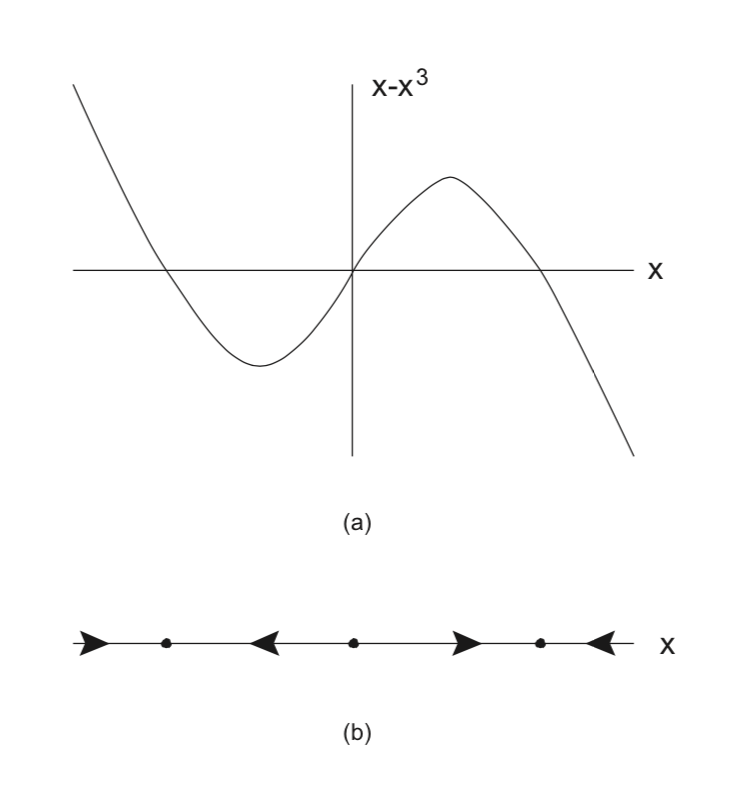
\[\dot{x} = x-x^3 = x(1-x^2), x \in \mathbb{R}. \label{2.12}\]
This vector field has three equilibrium points at \(x = 0, \pm 1\).
In Fig. 2.1 we show the graph of the vector field (2.12) in panel a) and the phase line dynamics in panel b).
The solid black dots in panel b) correspond to the equilibrium points and these, in turn, correspond to the zeros of the vector field shown in panel a). Between its zeros, the vector field has a fixed sign (i.e. positive or negative), corresponding to ẋ being either increasing or decreasing. This is indicated by the direction of the arrows in panel b).
Our discussion about trajectories, as well as this example, brings us to a point where it is natural to introduce the important notion of an invariant set. While this is a general idea that applies to both autonomous and nonautonomous systems, in this course we will only discuss this notion in the context of autonomous systems. Accordingly, let \(\phi_{t}(\cdot)\) denote the flow generated by an autonomous vector field.
DEFINITION 11: INVARIANT SET
A set \(M \subset \mathbb{R}^n\) is said to be invariant if
\[x \in M \Rightarrow \phi_{t}(x) \in M\]
\(\forall t\).
In other words, a set is invariant (with respect to a flow) if you start in the set, and remain in the set, forever.
If you think about it, it should be clear that invariant sets are sets of trajectories. Any single trajectory is an invariant set. The entire phase space is an invariant set. The most interesting cases are those ''in between''. Also, it should be clear that the union of any two invariant sets is also an invariant set (just apply the definition of invariant set to the union of two, or more, invariant sets).
There are certain situations where we will be interested in sets that are invariant only for positive time–positive invariant sets.
DEFINITION 12: POSITIVE INVARIANT SET
A set \(M \subset \mathbb{R}^n\) is said to be positive invariant if
\(x \in M \Rightarrow \phi_{t}(x) \in M\) \(\forall t>0\).
There is a similar notion of negative invariant sets, but the generalization of this from the definition of positive invariant sets should be obvious, so we will not write out the details.
Concerning example 8, the three equilibrium points are invariant sets, as well as the closed intervals \([-1, 0]\) and [0, 1]. Are there other invariant sets?