
5: Behavior Near Equilbria - Linearization
- Page ID
- 24158

\( \newcommand{\vecs}[1]{\overset { \scriptstyle \rightharpoonup} {\mathbf{#1}} } \)
\( \newcommand{\vecd}[1]{\overset{-\!-\!\rightharpoonup}{\vphantom{a}\smash {#1}}} \)
\( \newcommand{\dsum}{\displaystyle\sum\limits} \)
\( \newcommand{\dint}{\displaystyle\int\limits} \)
\( \newcommand{\dlim}{\displaystyle\lim\limits} \)
\( \newcommand{\id}{\mathrm{id}}\) \( \newcommand{\Span}{\mathrm{span}}\)
( \newcommand{\kernel}{\mathrm{null}\,}\) \( \newcommand{\range}{\mathrm{range}\,}\)
\( \newcommand{\RealPart}{\mathrm{Re}}\) \( \newcommand{\ImaginaryPart}{\mathrm{Im}}\)
\( \newcommand{\Argument}{\mathrm{Arg}}\) \( \newcommand{\norm}[1]{\| #1 \|}\)
\( \newcommand{\inner}[2]{\langle #1, #2 \rangle}\)
\( \newcommand{\Span}{\mathrm{span}}\)
\( \newcommand{\id}{\mathrm{id}}\)
\( \newcommand{\Span}{\mathrm{span}}\)
\( \newcommand{\kernel}{\mathrm{null}\,}\)
\( \newcommand{\range}{\mathrm{range}\,}\)
\( \newcommand{\RealPart}{\mathrm{Re}}\)
\( \newcommand{\ImaginaryPart}{\mathrm{Im}}\)
\( \newcommand{\Argument}{\mathrm{Arg}}\)
\( \newcommand{\norm}[1]{\| #1 \|}\)
\( \newcommand{\inner}[2]{\langle #1, #2 \rangle}\)
\( \newcommand{\Span}{\mathrm{span}}\) \( \newcommand{\AA}{\unicode[.8,0]{x212B}}\)
\( \newcommand{\vectorA}[1]{\vec{#1}} % arrow\)
\( \newcommand{\vectorAt}[1]{\vec{\text{#1}}} % arrow\)
\( \newcommand{\vectorB}[1]{\overset { \scriptstyle \rightharpoonup} {\mathbf{#1}} } \)
\( \newcommand{\vectorC}[1]{\textbf{#1}} \)
\( \newcommand{\vectorD}[1]{\overrightarrow{#1}} \)
\( \newcommand{\vectorDt}[1]{\overrightarrow{\text{#1}}} \)
\( \newcommand{\vectE}[1]{\overset{-\!-\!\rightharpoonup}{\vphantom{a}\smash{\mathbf {#1}}}} \)
\( \newcommand{\vecs}[1]{\overset { \scriptstyle \rightharpoonup} {\mathbf{#1}} } \)
\(\newcommand{\longvect}{\overrightarrow}\)
\( \newcommand{\vecd}[1]{\overset{-\!-\!\rightharpoonup}{\vphantom{a}\smash {#1}}} \)
\(\newcommand{\avec}{\mathbf a}\) \(\newcommand{\bvec}{\mathbf b}\) \(\newcommand{\cvec}{\mathbf c}\) \(\newcommand{\dvec}{\mathbf d}\) \(\newcommand{\dtil}{\widetilde{\mathbf d}}\) \(\newcommand{\evec}{\mathbf e}\) \(\newcommand{\fvec}{\mathbf f}\) \(\newcommand{\nvec}{\mathbf n}\) \(\newcommand{\pvec}{\mathbf p}\) \(\newcommand{\qvec}{\mathbf q}\) \(\newcommand{\svec}{\mathbf s}\) \(\newcommand{\tvec}{\mathbf t}\) \(\newcommand{\uvec}{\mathbf u}\) \(\newcommand{\vvec}{\mathbf v}\) \(\newcommand{\wvec}{\mathbf w}\) \(\newcommand{\xvec}{\mathbf x}\) \(\newcommand{\yvec}{\mathbf y}\) \(\newcommand{\zvec}{\mathbf z}\) \(\newcommand{\rvec}{\mathbf r}\) \(\newcommand{\mvec}{\mathbf m}\) \(\newcommand{\zerovec}{\mathbf 0}\) \(\newcommand{\onevec}{\mathbf 1}\) \(\newcommand{\real}{\mathbb R}\) \(\newcommand{\twovec}[2]{\left[\begin{array}{r}#1 \\ #2 \end{array}\right]}\) \(\newcommand{\ctwovec}[2]{\left[\begin{array}{c}#1 \\ #2 \end{array}\right]}\) \(\newcommand{\threevec}[3]{\left[\begin{array}{r}#1 \\ #2 \\ #3 \end{array}\right]}\) \(\newcommand{\cthreevec}[3]{\left[\begin{array}{c}#1 \\ #2 \\ #3 \end{array}\right]}\) \(\newcommand{\fourvec}[4]{\left[\begin{array}{r}#1 \\ #2 \\ #3 \\ #4 \end{array}\right]}\) \(\newcommand{\cfourvec}[4]{\left[\begin{array}{c}#1 \\ #2 \\ #3 \\ #4 \end{array}\right]}\) \(\newcommand{\fivevec}[5]{\left[\begin{array}{r}#1 \\ #2 \\ #3 \\ #4 \\ #5 \\ \end{array}\right]}\) \(\newcommand{\cfivevec}[5]{\left[\begin{array}{c}#1 \\ #2 \\ #3 \\ #4 \\ #5 \\ \end{array}\right]}\) \(\newcommand{\mattwo}[4]{\left[\begin{array}{rr}#1 \amp #2 \\ #3 \amp #4 \\ \end{array}\right]}\) \(\newcommand{\laspan}[1]{\text{Span}\{#1\}}\) \(\newcommand{\bcal}{\cal B}\) \(\newcommand{\ccal}{\cal C}\) \(\newcommand{\scal}{\cal S}\) \(\newcommand{\wcal}{\cal W}\) \(\newcommand{\ecal}{\cal E}\) \(\newcommand{\coords}[2]{\left\{#1\right\}_{#2}}\) \(\newcommand{\gray}[1]{\color{gray}{#1}}\) \(\newcommand{\lgray}[1]{\color{lightgray}{#1}}\) \(\newcommand{\rank}{\operatorname{rank}}\) \(\newcommand{\row}{\text{Row}}\) \(\newcommand{\col}{\text{Col}}\) \(\renewcommand{\row}{\text{Row}}\) \(\newcommand{\nul}{\text{Nul}}\) \(\newcommand{\var}{\text{Var}}\) \(\newcommand{\corr}{\text{corr}}\) \(\newcommand{\len}[1]{\left|#1\right|}\) \(\newcommand{\bbar}{\overline{\bvec}}\) \(\newcommand{\bhat}{\widehat{\bvec}}\) \(\newcommand{\bperp}{\bvec^\perp}\) \(\newcommand{\xhat}{\widehat{\xvec}}\) \(\newcommand{\vhat}{\widehat{\vvec}}\) \(\newcommand{\uhat}{\widehat{\uvec}}\) \(\newcommand{\what}{\widehat{\wvec}}\) \(\newcommand{\Sighat}{\widehat{\Sigma}}\) \(\newcommand{\lt}{<}\) \(\newcommand{\gt}{>}\) \(\newcommand{\amp}{&}\) \(\definecolor{fillinmathshade}{gray}{0.9}\)Now we will consider several examples for solving, and understanding, the nature of the solutions, of
\[\dot{x} = Ax, x \in \mathbb{R}^2. \label{5.1}\]
For all of the examples, the method for solving the system is the same.
Steps for Solving
- Step 1. Compute the eigenvalues of \(A\).
- Step 2. Compute the eigenvectors of \(A\).
- Step 3. Use the eigenvectors of \(A\) to form the transformation matrix \(T\).
- Step 4. Compute \(\Lambda = T^{-1}AT\).
- Step 5. Compute \(e^{At} = Te^{\lambda t}T^{-1}\).
Once we have computed \(e^{At}\) we have the solution of Equation \ref{5.1} through any initial condition \(y_{0}\) since \(y(t)\), \(y(0) = y_{0}\), is given by \(y(t) = e^{At}y_{0}\).
Example \(\PageIndex{10}\)
We consider the following linear, autonomous ODE:
\[\begin{pmatrix} {\dot{x_{1}}}\\ {\dot{x_{2}}} \end{pmatrix} = \begin{pmatrix} {2}&{1}\\ {1}&{2} \end{pmatrix} \begin{pmatrix} {x_{1}}\\ {x_{2}} \end{pmatrix} \label{5.2}\]
where
\[A = \begin{pmatrix} {2}&{1}\\ {1}&{2} \end{pmatrix}, \label{5.3}\]
Step 1. Compute the eigenvalues of A.
The eigenvalues of A, denote by \(\lambda\), are given by the solutions of the characteristic polynomial:
\(det \begin{pmatrix} {2-\lambda}&{1}\\ {1}&{2-\lambda} \end{pmatrix} = (2-\lambda)^2-1 = 0\)
\[= \lambda^{2}-4\lambda+3 = 0, \label{5.4}\]
or
\(\lambda_{1,2} = 2 \pm \frac{1}{2}\sqrt{16-12} = 3, 1\)
Step 2. Compute the eigenvectors of A.
For each eigenvalue, we compute the corresponding eigenvector. The eigenvector corresponding to the eigenvalue 3 is found by solving:
\[\begin{pmatrix} {2}&{1}\\ {1}&{2} \end{pmatrix} \begin{pmatrix} {x_{1}}\\ {x_{2}} \end{pmatrix} = 3\begin{pmatrix} {x_{1}}\\ {x_{2}} \end{pmatrix}, \label{5.5}\]
or
\[2x_{1}+x_{2} = 3x_{1}, \label{5.6}\]
\[x_{1}+2x_{2} = 3x_{2}. \label{5.7}\]
Both of these equations yield the same equation since the two equations are dependent:
\[x_{2} = x_{1} \label{5.8}\].
Therefore we take as the eigenvector corresponding to the eigenvalue 3:
\[\begin{pmatrix} {1}\\ {1} \end{pmatrix} \label{5.9}\]
Next we compute the eigenvector corresponding to the eigenvalue 1. This is given by a solution to the following equations:
\[\begin{pmatrix} {2}&{1}\\ {1}&{2} \end{pmatrix} \begin{pmatrix} {x_{1}}\\ {x_{2}} \end{pmatrix} = \begin{pmatrix} {x_{1}}\\ {x_{2}} \end{pmatrix}, \label{5.10}\]
or
\[2x_{1}+x_{2} = x_{1}, \label{5.11}\]
\[x_{1}+2x_{2} = x_{2}. \label{5.12}\]
Both of these equations yield the same equation:
\[x_{2} = -x_{1}. \label{5.13}\]
Therefore we take as the eigenvector corresponding to the eigenvalue:
\[\begin{pmatrix} {1}\\ {-1} \end{pmatrix} \label{5.14}\]
Step 3. Use the eigenvectors of A to form the transformation matrix T.
For the columns of \(T\) we take the eigenvectors corresponding the the eigenvalues 1 and 3:
\[T = \begin{pmatrix} {1}&{1}\\ {-1}&{1} \end{pmatrix} \label{5.15}\]
with the inverse given by:
\[T^{-1} = \frac{1}{2}\begin{pmatrix} {1}&{-1}\\ {1}&{1} \end{pmatrix} \label{5.16}\]
Step 4. Compute \(\Lambda = T^{-1}AT\).
We have:
\(T^{-1}AT = \dfrac{1}{2}\begin{pmatrix} {1}&{-1}\\ {1}&{1} \end{pmatrix} \begin{pmatrix} {2}&{1}\\ {1}&{2} \end{pmatrix} \begin{pmatrix} {1}&{1}\\ {-1}&{1} \end{pmatrix}\)
\( = \frac{1}{2}\begin{pmatrix} {1}&{-1}\\ {1}&{1} \end{pmatrix} \begin{pmatrix} {1}&{3}\\ {-1}&{3} \end{pmatrix}\)
\[= \begin{pmatrix} {1}&{0}\\ {0}&{3} \end{pmatrix} \equiv \Lambda \label{5.17}\]
Therefore, in the \(u_{1}-u_{2}\) coordinates (5.2) becomes:
\[\begin{pmatrix} {\dot{u_{1}}}\\ {\dot{u_{2}}} \end{pmatrix} = \begin{pmatrix} {1}&{0}\\ {0}&{3} \end{pmatrix} \begin{pmatrix} {u_{1}}\\ {u_{2}} \end{pmatrix} \label{5.18}\]
In the \(u_{1}-u_{2}\) coordinates it is easy to see that the origin is an unstable equilibrium point.
Step 5. Compute \(e^{At} = Te^{\lambda t}T^{-1}\).
We have:
\(e^{AT} = \frac{1}{2}\begin{pmatrix} {1}&{1}\\ {-1}&{1} \end{pmatrix} \begin{pmatrix} {e^{t}}&{0}\\ {0}&{e^{3t}} \end{pmatrix} \begin{pmatrix} {1}&{-1}\\ {1}&{1} \end{pmatrix}\)
\(= \frac{1}{2}\begin{pmatrix} {1}&{1}\\ {-1}&{1} \end{pmatrix} \begin{pmatrix} {e^{t}}&{-e^{t}}\\ {e^{3t}}&{e^{3t}} \end{pmatrix}\)
\[= \begin{pmatrix} \frac{1}{2}{e^{t}+e^{3t}}&{-e^{t}+e^{3t}}\\ {-e^{t}+e^{3t}}&{e^{t}+e^{3t}} \end{pmatrix} \label{5.19}\]
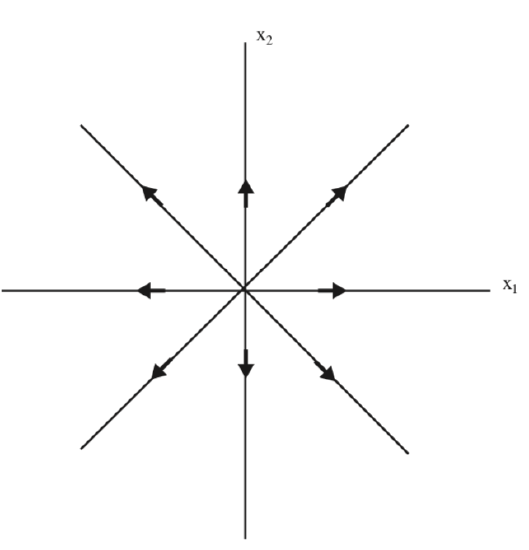
We see that the origin is also unstable in the original \(x_{1}-x_{2}\) coordinates. It is referred to as a source, and this is characterized by the fact that all of the eigenvalues of A have positive real part. The phase portrait is illustrated in Fig. 5.1.
We remark this it is possible to infer the behavior of \(e^{At}\) as \(t \rightarrow \infty\) from the behavior of \(e^{\Lambda t}\) as \(t \rightarrow \infty\) since T does not depend on t.
Example \(\PageIndex{11}\)
We consider the following linear, autonomous ODE:
\[\begin{pmatrix} {\dot{x_{1}}}\\ {\dot{x_{2}}} \end{pmatrix} = \begin{pmatrix} {-1}&{-1}\\ {9}&{-1} \end{pmatrix} \begin{pmatrix} {x_{1}}\\ {x_{2}} \end{pmatrix} \label{5.20}\]
where
\[A = \begin{pmatrix} {-1}&{-1}\\ {9}&{-1} \end{pmatrix}, \label{5.21}\]
Step 1. Compute the eigenvalues of A.
The eigenvalues of A, denote by \(\lambda\), are given by the solutions of the characteristic polynomial:
\(det \begin{pmatrix} {-1-\lambda}&{-1}\\ {9}&{-1-\lambda} \end{pmatrix} = (-1-\lambda)^2+9 = 0\),
\[= \lambda^{2}+2\lambda+10 = 0, \label{5.22}\]
or
\(\lambda_{1,2} = -1 \pm \frac{1}{2}\sqrt{4-40} = -1 \pm 3i\)
The eigenvectors are complex, so we know it is not diagonalizable over the real numbers. What this means is that we cannot find real eigenvectors so that it can be transformed to a form where there are real numbers on the diagonal, and zeros in the off diagonal entries. The best we can do is to transform it to a form where the real parts of the eigenvalue are on the diagonal, and the imaginary parts are on the off diagonal locations, but the off diagonal elements differ by a minus sign.
Step 2. Compute the eigenvectors of A.
The eigenvector of A corresponding to the eigenvector \(-1-3i\) is the solution of the following equations:
\[\begin{pmatrix} {-1}&{-1}\\ {9}&{-1} \end{pmatrix} \begin{pmatrix} {x_{1}}\\ {x_{2}} \end{pmatrix} = (-1-3i) \begin{pmatrix} {x_{1}}\\ {x_{2}} \end{pmatrix}, \label{5.23}\]
or
\[-x_{1}-x_{2} = -x_{1}-3ix_{2}, \label{5.24}\]
\[9x_{1}-x_{2} = -x_{2}-3ix_{2}. \label{5.25}\]
A solution to these equations is given by:
\(\begin{pmatrix} {1}\\ {3i} \end{pmatrix} = \begin{pmatrix} {1}\\ {0} \end{pmatrix}+i \begin{pmatrix} {0}\\ {3} \end{pmatrix}\)
Step 3. Use the eigenvectors of A to form the transformation matrix T.
For the first column of T we take the real part of the eigenvector corresponding to the eigenvalue \(-1-3i\), and for the second column we take the complex part of the eigenvector:
\[T = \begin{pmatrix} {1}&{0}\\ {0}&{3} \end{pmatrix} \label{5.26}\]
with the inverse given by:
\[T^{-1} = \begin{pmatrix} {1}&{0}\\ {0}&{\frac{1}{3}} \end{pmatrix} \label{5.27}\]
Step 4. Compute \(\Lambda = T^{-1}AT\).
\(T^{-1}AT = \frac{1}{2}\begin{pmatrix} {1}&{0}\\ {0}&{\frac{1}{3}} \end{pmatrix} \begin{pmatrix} {-1}&{-1}\\ {9}&{-1} \end{pmatrix} \begin{pmatrix} {1}&{0}\\ {0}&{3} \end{pmatrix}\)
\(= \begin{pmatrix} {1}&{0}\\ {0}&{\frac{1}{3}} \end{pmatrix} \begin{pmatrix} {-1}&{-3}\\ {9}&{-3} \end{pmatrix}\)
\[= \begin{pmatrix} {-1}&{-3}\\ {3}&{-1} \end{pmatrix} \equiv \Lambda \label{5.28}\]
With \(\Lambda\) in this form, we know from the previous chapter that:
\[e^{\Lambda t} = e^{-t}\begin{pmatrix} {cos3t}&{-sin3t}\\ {sin3t}&{cos3t} \end{pmatrix} \label{5.29}\]
Then we have:
\(e^{At} = Te^{\Lambda t}T^{-1}\).
From this expression we can conclude that \(e^{At} \rightarrow 0\) as \(t \rightarrow \infty\). Hence the origin is asymptotically stable. It is referred to as a sink and it is characterized by the real parts of the eigenvalues of A being negative. The phase plane is sketched in Fig. 5.2.

Example \(\PageIndex{12}\)
We consider the following linear, autonomous ODE:
\[\begin{pmatrix} {\dot{x_{1}}}\\ {\dot{x_{2}}} \end{pmatrix} = \begin{pmatrix} {-1}&{1}\\ {1}&{1} \end{pmatrix} \begin{pmatrix} {x_{1}}\\ {x_{2}} \end{pmatrix} \label{5.30}\]
where
\[A = \begin{pmatrix} {-1}&{1}\\ {1}&{1} \end{pmatrix}, \label{5.31}\]
Step 1. Compute the eigenvalues of A.
The eigenvalues of A, denote by \(\lambda\), are given by the solutions of the characteristic polynomial:
\(det \begin{pmatrix} {-1-\lambda}&{1}\\ {1}&{1-\lambda} \end{pmatrix} = (-1-\lambda)(1-\lambda)-1 = 0\)
\[= \lambda^{2}-2 = 0, \label{5.32}\]
which are
\(\lambda_{1,2} = \pm\sqrt{2}\)
Step 2. Compute the eigenvectors of A.
The eigenvector corresponding to the eigenvalue \(\sqrt{2}\) is given by the solution of the following equations:
\[\begin{pmatrix} {-1}&{1}\\ {1}&{1} \end{pmatrix} \begin{pmatrix} {x_{1}}\\ {x_{2}} \end{pmatrix} = \sqrt{2}\begin{pmatrix} {x_{1}}\\ {x_{2}} \end{pmatrix}, \label{5.33}\]
or
\[-x_{1}+x_{2} = \sqrt{2}x_{1}, \label{5.34}\]
\[x_{1}+x_{2} = \sqrt{2}x_{2}. \label{5.35}\]
A solution is given by:
\(x_{2} = (1+\sqrt{2})x_{1}\).
corresponding to the eigenvector
\(\begin{pmatrix} {1}\\ {1+\sqrt{2}} \end{pmatrix}\)
The eigenvector corresponding to the eigenvalue \(-\sqrt{2}\) is given by the solution to the following equations:
\[\begin{pmatrix} {-1}&{1}\\ {1}&{1} \end{pmatrix} \begin{pmatrix} {x_{1}}\\ {x_{2}} \end{pmatrix} = -\sqrt{2}\begin{pmatrix} {x_{1}}\\ {x_{2}} \end{pmatrix}, \label{5.36}\]
or
\[-x_{1}+x_{2} = -\sqrt{2}x_{1}, \label{5.37}\]
\[x_{1}+x_{2} = -\sqrt{2}x_{2}. \label{5.38}\]
A solution is given by:
\(x_{2} = (1-\sqrt{2})x_{1}\).
corresponding to the eigenvector:
\(\begin{pmatrix} {1}\\ {1-\sqrt{2}} \end{pmatrix}\)
Step 3. Use the eigenvectors of A to form the transformation matrix T.
For the columns of T we take the eigenvectors corresponding the the eigenvalues \(\sqrt{2}\) and \(-\sqrt{2}\):
\[T = \begin{pmatrix} {1}&{1}\\ {1+\sqrt{2}}&{1-\sqrt{2}} \end{pmatrix} \label{5.39}\]
with the inverse given by:
\[T^{-1} = -\frac{1}{2\sqrt{2}}\begin{pmatrix} {1-\sqrt{2}}&{-1}\\ {-1-\sqrt{2}}&{1} \end{pmatrix} \label{5.40}\]
Step 4. Compute \(\Lambda = T^{-1}AT\).We have:
\(T^{-1}AT = -\frac{1}{2\sqrt{2}}\begin{pmatrix} {1-\sqrt{2}}&{-1}\\ {-1-\sqrt{2}}&{1} \end{pmatrix} \begin{pmatrix} {-1}&{1}\\ {1}&{1} \end{pmatrix} \begin{pmatrix} {1}&{1}\\ {1+\sqrt{2}}&{1-\sqrt{2}} \end{pmatrix}\)
\(= -\frac{1}{2\sqrt{2}}\begin{pmatrix} {1-\sqrt{2}}&{-1}\\ {-1-\sqrt{2}}&{1} \end{pmatrix} \begin{pmatrix} {\sqrt{2}}&{-\sqrt{2}}\\ {2+\sqrt{2}}&{2-\sqrt{2}} \end{pmatrix}\)
\[= \begin{pmatrix} {\sqrt{2}}&{0}\\ {0}&{-\sqrt{2}} \end{pmatrix} \equiv \Lambda \label{5.41}\]
Therefore, in the \(u_{1}-u_{2}\) coordinates (5.30) becomes:
\[\begin{pmatrix} {\dot{u_{1}}}\\ {\dot{u_{2}}} \end{pmatrix} = \begin{pmatrix} {\sqrt{2}}&{0}\\ {0}&{-\sqrt{2}} \end{pmatrix} \begin{pmatrix} {u_{1}}\\ {u_{2}} \end{pmatrix} \label{5.42}\]
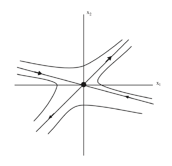
The phase portrait of (5.42) is shown in 5.3.
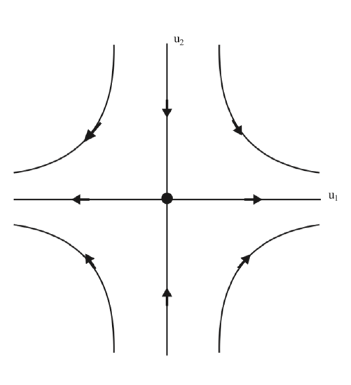
It is easy to see that the origin is unstable for (5.42). In fig. 5.3 we see that the origin has the structure of a saddle point, and we want to explore this idea further.
In the \(u_{1}-u_{2}\) coordinates the span of the eigenvector corresponding to the eigenvalue \(\sqrt{2}\) is given by \(u_{2} = 0\), i.e. the \(u_{1}\) axis. The span of the eigenvector corresponding to the eigenvalue \(-\sqrt{2}\) is given by \(u_{1} = 0\), i.e. the \(u_{2}\) axis. Moreover, we can see from the form of (5.42) that these coordinate axes are invariant. The \(u_{1}\) axis is referred to as the unstable subspace, denoted by \(E^{u}\), and the \(u_{2}\) axis is referred to as the stable subspace, denoted by \(E^{s}\). In other words, the unstable subspace is the span of the eigenvector corresponding to the eigenvalue with positive real part and the stable subspace is the span of the eigenvector corresponding to the eigenvalue having negative real part. The stable and unstable subspaces are invariant subspaces with respect to the flow generated by (5.42).
The stable and unstable subspaces correspond to the coordinate axes in the coordinate system given by the eigenvectors. Next we want to understand how they would appear in the original \(x_{1}-x_{2}\) coordinates. This is accomplished by transforming them to the original coordinates using the transformation matrix (Equation \ref{5.39}).
We first transform the unstable subspace from the \(u_{1}-u_{2}\) coordinates to the \(x_{1}-x_{2}\) coordinates. In the \(u_{1}-u_{2}\) coordinates points on the unstable subspace have coordinates \((u_{1}, 0)\). Acting on these points with T gives:
\[T\begin{pmatrix} {u_{1}}\\ {0} \end{pmatrix} = \begin{pmatrix} {1}&{1}\\ {1+\sqrt{2}}&{1-\sqrt{2}} \end{pmatrix} \begin{pmatrix} {u_{1}}\\ {0} \end{pmatrix} = \begin{pmatrix} {x_{1}}\\ {x_{2}} \end{pmatrix}, \label{5.43}\]
which gives the following relation between points on the unstable subspace in the \(u_{1}-u_{2}\) coordinates to points in the \(x_{1}-x_{2}\) coordinates:
\[u_{1} = x_{1}, \label{5.44}\]
\[(1+\sqrt{2})u_{1} = x_{2}, \label{5.45}\]
or
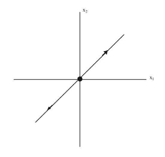
\[(1 + \sqrt{2})x_{1} = x_{2}. \label{5.46}\]
This is the equation for the unstable subspace in the \(x_{1}-x_{2}\) coordinates, which we illustrate in Fig. 5.4.
Next we transform the stable subspace from the \(u_{1}-u_{2}\) coordinates to the \(x_{1}-x_{2}\) coordinates. In the \(u_{1}-u_{2}\) coordinates points on the stable subspace have coordinates \((0, u_{2})\). Acting on these points with T gives:
\[T\begin{pmatrix} {0}\\ {u_{2}} \end{pmatrix} = \begin{pmatrix} {1}&{1}\\ {1+\sqrt{2}}&{1-\sqrt{2}} \end{pmatrix} \begin{pmatrix} {0}\\ {u_{2}} \end{pmatrix} = \begin{pmatrix} {x_{1}}\\ {x_{2}} \end{pmatrix}, \label{5.47}\]
which gives the following relation between points on the stable subspace in the \(u_{1}-u_{2}\) coordinates to points in the \(x_{1}-x_{2}\) coordinates:
\[u_{2} = x_{1}, \label{5.48}\]
\[(1-\sqrt{2})u_{2} = x_{2}, \label{5.49}\]
or
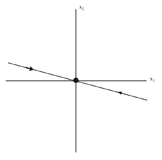
\[(1-\sqrt{2})x_{1} = x_{2}. \label{5.50}\]
This is the equation for the stable subspace in the \(x_{1}-x_{2}\) coordinates, which we illustrate in Fig. 5.5.
In Fig. 5.6 we illustrate both the stable and the unstable subspaces in the original coordinates.
Now we want to discuss some general results from these three examples.
For all three examples, the real parts of the eigenvalues of A were nonzero, and stability of the origin was determined by the sign of the real parts of the eigenvalues, e.g., for example 10 the origin was unstable (the real parts of the eigenvalues of A were positive), for example 11 the origin was stable (the real parts of the eigenvalues of A were negative), and for example 12 the origin was unstable (A had one positive eigenvalue and one negative eigenvalue). This is generally true for all linear, autonomous vector fields. We state this more formally.
Consider a linear, autonomous vector field on \(\mathbb{R}^n\):
\[\dot{y} = Ay, y(0) = y_{0}, y \in \mathbb{R}^n. \label{5.51}\]
Then if A has no eigenvalues having zero real parts, the stability of the origin is determined by the real parts of the eigenvalues of A. If all of the real parts of the eigenvalues are strictly less than zero, then the origin is asymptotically stable. If at least one of the eigenvalues of A has real part strictly larger than zero, then the origin is unstable.
There is a term applied to this terminology that permeates all of dynamical systems theory.
DEFINITION 20: HYPERBOLIC EQUILIBRIUM POINT
The origin of Equation \ref{5.51} is said to be if none of the real parts of the eigenvalues of A have zero real parts.
It follows that hyperbolic equilibria of linear, autonomous vector fields on \(\mathbb{R}^n\) can be either sinks, sources, or saddles. The key point is that the eigenvalues of A all have nonzero real parts.
If we restrict ourselves to two dimensions, it is possible to make a (short) list of all of the distinct canonical forms for A. These are given by the following six \(2 \times 2\) matrices.
The first is a diagonal matrix with real, nonzero eigenvalues \(\lambda, \mu \ne 0\), i.e. the origin is a hyperbolic fixed point:
\[\begin{pmatrix} {\lambda}&{0}\\ {0}&{\mu} \end{pmatrix} \label{5.52}\]
In this case the orgin can be a sink if both eigenvalues are negative, a source if both eigenvalues are positive, and a saddle if the eigenvalues have opposite sign.
The next situation corresponds to complex eigenvalues, with the real part, \(\alpha\), and imaginary part, \(\beta\), both being nonzero. In this case the equilibrium point is hyperbolic, and \(\alpha\) sink for \(\alpha < 0\), and a source for \(\alpha > 0\). The sign of \(\beta\) does not influence stability:
\[\begin{pmatrix} {\alpha}&{\beta}\\ {\beta}&{-\alpha} \end{pmatrix} \label{5.53}\]
Next we consider the case when the eigenvalues are real, identical, and nonzero, but the matrix is nondiagonalizable, i.e. two eigenvectors cannot be found. In this case the origin is hyperbolic for \(\lambda \ne 0\), and is a sink for \(\lambda < 0\) and a source for \(\lambda > 0\):
\[\begin{pmatrix} {\lambda}&{1}\\ {0}&{\lambda} \end{pmatrix} \label{5.54}\]
Next we consider some cases corresponding to the origin being nonhyperbolic that would have been possible to include in the discussion of earlier cases, but it is more instructive to explicitly point out these cases separately.
We first consider the case where A is diagonalizable with one nonzero real eigenvalue and one zero eigenvalue:
\[\begin{pmatrix} {\lambda}&{0}\\ {0}&{0} \end{pmatrix} \label{5.55}\]
We consider the case where the two eigenvalues are purely imaginary, \(\pm i\sqrt{b}\). In this case the origin is ref!erred to as a center.
\[\begin{pmatrix} {0}&{\beta}\\ {-\beta}&{0} \end{pmatrix} \label{5.56}\]
For completeness, we consider the case where both eigenvalues are zero and A is diagonal.
\[\begin{pmatrix} {0}&{0}\\ {0}&{0} \end{pmatrix} \label{5.57}\]
Finally, we want to expand on the discussion related to the geometrical aspects of Example 12. Recall that for that example the span of the eigenvector corresponding to the eigenvalue with negative real part was an invariant subspace, referred to as the stable subspace. Trajectories with initial conditions in the stable subspace decayed to zero at an exponential rate as \(t \rightarrow +\infty\). The stable invariant subspace was denoted by \(E^s\). Similarly, the span of the eigenvector corresponding to the eigenvalue with positive real part was an invariant subspace, referred to as the unstable subspace. Trajectories with initial conditions in the unstable subspace decayed to zero at an exponential rate as \(t \rightarrow -\infty\). The unstable invariant subspace was denoted by \(E^{u}\).
We can easily see that Equation \ref{5.52} has this behavior when \(\lambda\) and \(\mu\) have opposite signs. If \(\lambda\) and \(\mu\) are both negative, then the span of the eigenvectors corresponding to these two eigenvalues is \(\mathbb{R}^2\), and the entire phase space is the stable subspace. Similarly, if \(\lambda\) and \(\mu\) are both positive, then the span of the eigenvectors corresponding to these two eigenvalues is \(\mathbb{R}^2\), and the entire phase space is the unstable subspace.
The case Equation \ref{5.53} is similar. For that case there is not a pair of real eigenvectors corresponding to each of the complex eigenvalues. The vectors that transform the original matrix to this canonical form are referred to as generalized eigenvectors. If \(\alpha < 0\) the span of the generalized eigenvectors is \(\mathbb{R}^2\), and the entire phase space is the stable subspace. Similarly, if \(\alpha > 0\) the span of the generalized eigenvectors is \(\mathbb{R}^2\), and the entire phase space is the unstable subspace. The situation is similar for (5.54). For \(\lambda < 0\) the entire phase space is the stable subspace, for \(\lambda > 0\) the entire phase space is the unstable subspace.
The case in Equation \ref{5.55} is different. The span of the eigenvector corresponding to \(\lambda\) is the stable subspace for \(\lambda < 0\), and the unstable subspace for \(\lambda > 0\) The space of the eigenvector corresponding to the zero eigenvalue is referred to as the center subspace.
For the case (5.56) there are not two real eigenvectors leading to the resulting canonical form. Rather, there are two generalized eigenvectors associated with this pair of complex eigenvalues having zero real part. The span of these two eigenvectors is a two dimensional center subspace corresponding to \(\mathbb{R}^2\). An equilibrium point with purely imaginary eigenvalues is referred to as a center.
Finally, the case in Equation \ref{5.57} is included for completeness. It is the zero vector field where \(\mathbb{R}^2\) is the center subspace.
We can characterize stability of the origin in terms of the stable, unstable, and center subspaces. The origin is asymptotically stable if \(E^u = \emptyset\) and \(E^c = \emptyset\).The origin is unstable if \(E^u \ne \emptyset\).