4: Behavior Near Trajectories - Linearization

Now we are going to discuss a method for analyzing stability that utilizes linearization about the object whose stability is of interest. For now, the "objects of interest" are specific solutions of a vector field.The structure of the solutions of linear, constant coefficient systems is covered in many ODE textbooks. My favorite is the book of Hirsch et al.1. It covers all of the linear algebra needed for analyzing linear ODEs that you probably did not cover in your linear algebra course. The book by Arnold is also very good, but the presentation is more compact, with fewer examples.

We begin by considering a general nonautonomous vector field:

\[\dot{x} = f(x, t), x \in \mathbb{R}^n, \label{4.1}\]

and we suppose that

\[\bar{x}(t, t_{0}, x_{0}), \label{4.2}\]

is the solution of Equation \ref{4.1} for which we wish to determine its stability properties. As when we introduced the definitions of stability, we proceed by localizing the vector field about the solution of interest. We do this by introducing the change of coordinates

\(x = y+\bar{x}\)

for Equation \ref{4.1} as follows:

\(\dot{x} = \dot{y}+\dot{\bar{x}} = f(y+\bar{x}, t)\),

or

\(\dot{y} = f(y+\bar{x}, t)\dot{\bar{x}}\),

\[= f(y+\bar{x}, t)f(\bar{x}, t), \label{4.3}\]

where we omit the arguments of \(\bar{x}(t, t_{0}, x_{0})\) for the sake of a less cumbersome notation. Next we Taylor expand \(f(y+\bar{x}, t)\) in \(y\) about the solution \(\bar{x}\), but we will only require the leading order terms explicitly

\[f(y+\bar{x}, t) = f(\bar{x}, t)+Df(\bar{x},t)y+\mathbb{O}(|y|^2), \label{4.4}\]

where \(Df\) denotes the derivative (i.e. Jacobian matrix) of the vector valued function f and \(\mathbb{O}(|y|^2)\) denotes higher order terms in the Taylor expansion that we will not need in explicit form. Substituting this into Equation \ref{4.4} gives:

\(\dot{y} = f(y+\bar{x}, t) - f(\bar{x}, t)\),

\(= f(\bar{x}, t)+Df(\bar{x}, t)y+\mathbb{O}(|y|^2)f(\bar{x}, t)\),

\[= Df(\bar{x}, t)y+\mathbb{O}(|y|^2). \label{4.5}\]

Keep in mind that we are interested in the behavior of solutions near \(\bar{x}(t, t_{0}, x_{0})\), i.e., for \(y\) small. Therefore, in that situation it seems reasonable that neglecting the \(\mathbb{O}(|y|^2)\) in Equation \ref{4.5} would be an approximation that would provide us with the particular information that we seek. For example, would it provide sufficient information for us to deter- mine stability? In particular,

\[\dot{y} = Df(\bar{x}, t)y, \label{4.6}\]

is referred to as the linearization of the vector field \(\dot{x} = f (x, t)\) about the solution \(\bar{x}(t, t_{0}, x_{0})\).

Before we answer the question as to whether or not Equation \ref{4.1} provides an adequate approximation to solutions of Equation \ref{4.5} for y "small", we will first study linear vector fields on their own.

Linear vector fields can also be classified as nonautonomous or autonomous. Nonautonomous linear vector fields are obtained by linearizing a nonautonomous vector field about a solution (and retaining only the linear terms). They have the general form:

\[\dot{y} = A(t)y, y(0) = y_{0}, \label{4.7}\]

where

\[A(t) \equiv Df(\bar{x}(t, t_{0}, x_{0}), t) \label{4.8}\]

is a \(n \times n\) matrix. They can also be obtained by linearizing an autonomous vector field about a time-dependent solution.

An autonomous linear vector field is obtained by linearizing an autonomous vector field about an equilibrium point. More precisely, let \(\dot{x} = f(x)\) denote an autonomous vector field and let \(x = x_{0}\) denote an equilibrium point, i.e. \(f(x_{0}) = 0\). The linearized autonomous vector field about this equilibrium point has the form:

\[\dot{y} = Df(x_{0})y, y(0) = y_{0}, \label{4.9}\]

or

\[\dot{y} = Ay, y(0) = y_{0}, \label{4.10}\]

where \(A \equiv Df(x_{0})\) is a \(n \times n\) matrix of real numbers. This is significant because (4.10) can be solved using techniques of linear algebra, but Equation \ref{4.7}, generally, cannot be solved in this manner. Hence, we will now describe the general solution of (4.10).

The general solution of Equation \ref{4.10} is given by:

\[y(t) = e^{At}y_{0}. \label{4.11}\]

In order to verify that this is the solution, we merely need to substitute into the right hand side and the left hand side of (4.10) and show that equality holds. However, first we need to explain what \(e^{At}\) is, i.e. the exponential of the \(n \times n\) matrix A (by examining Equation \ref{4.11} it should be clear that if Equation \ref{4.11} is to make sense mathematically, then \(e^{At}\) must be a \(n times n\) matrix).

Just like the exponential of a scalar, the exponential of a matrix is defined through the exponential series as follows:

\(e^{At} \equiv \mathbb{I}+At+\frac{1}{2!}A^{2}t^{2}+···+\frac{1}{n!}A^{n}t^{n}+\cdots\),

\[= \sum_{i=0}^{n}\frac{1}{i!}A^{i}t^{i}, \label{4.12}\]

where \(\mathbb{I}\) denotes the \(n \times n\) identity matrix. But we still must answer the question, "does this exponential series involving products of matrices make mathematical sense"? Certainly we can compute products of matrices and multiply them by scalars. But we have to give meaning to an infinite sum of such mathematical objects. We do this by defining the norm of a matrix and then considering the convergence of the series in norm. When this is done the "convergence problem" is exactly the same as that of the exponential of a scalar. Therefore the exponential series for a matrix converges absolutely for all t, and therefore it can be differentiated with respect to t term-by-term, and the resulted series of derivatives also converges absolutely.

Next we need to argue that Equation \ref{4.11} is a solution of Equation \ref{4.10}. If we differentiate the series (4.12) term by term, we obtain that:

\[\frac{d}{dt}e^{At} = Ae^{At} = e^{At}A, \label{4.13}\]

where we have used the fact that the matrices A and \(e^{At}\) commute (this is easy to deduce from the fact that A commutes with any power of A) It then follows from this calculation that:

\[\dot{y} = \frac{d}{dt}e^{At}y_{0} = Ae^{At}y_{0} = Ay. \label{4.14}\]

Therefore the general problem of solving (4.10) is equivalent to computing \(e^{At}\), and we now turn our attention to this task.

First, suppose that \(A\) is a diagonal matrix, say

\[A = \begin{pmatrix} {\lambda_{1}}&{0}&{\cdots}&{0}\\ {0}&{\lambda_{2}}&{\cdots}&{0}\\ {0}&{0}&{\cdots}&{0}\\ {0}&{0}&{\cdots}&{\lambda_{n}} \end{pmatrix} \label{4.15}\]

Then it is easy to see by substituting A into the exponential series (4.12) that:

\[e^{At} = \begin{pmatrix} {e^{\lambda_{1}t}}&{0}&{\cdots}&{0}\\ {0}&{e^{\lambda_{2}t}}&{\cdots}&{0}\\ {0}&{0}&{\cdots}&{0}\\ {0}&{0}&{\cdots}&{e^{\lambda}t} \end{pmatrix} \label{4.16}\]

Therefore our strategy will be to transform coordinates so that in the new coordinates A becomes diagonal (or as "close as possible" to diagonal, which we will explain shortly). Then \(e^{At}\) will be easily computable in these coordinates. Once that is accomplished, then we use the inverse of the transformation to transform the solution back to the original coordinate system.

Now we make these ideas precise. We let

\[y = Tu, u \in \mathbb{R}^n, y \in \mathbb{R}^n, \label{4.17}\]

where T is a \(n \times n\) matrix whose precise properties will be developed in the following.

This is a typical approach in ODEs. We propose a general coordinate transformation of the ODE, and then we construct it in a way that gives the properties of the ODE that we desire. Substituting (4.17) into (4.10) gives:

\[\dot{y} = T\dot{u} = Ay = ATu, \label{4.18}\]

T will be constructed in a way that makes it invertible, so that we have:

\[\dot{u} = T^{-1}ATu, u(0) = T^{-1}y(0). \label{4.19}\]

To simplify the notation we let:

\[T = T^{-1}AT, \label{4.20}\]

or

\[A = T^{-1}\Lambda T. \label{4.21}\]

Substituting (4.21) into the series for the matrix exponential (4.12) gives:

\(e^{At} = e^{T\Lambda T^{-1}t}\),

\[= \mathbb{1}+ T\Lambda T^{-1}t+\frac{1}{2!}(T\Lambda T^{-1})^{2}t^2+\cdots+\frac{1}{n!}(T\Lambda T^{-1})^{n}t^n+\cdots \label{4.22}\]

Now note that for any positive integer n we have:

\((T\Lambda T^{-1})^{n} = \underbrace{(T\Lambda T^{-1})(T\Lambda T^{-1})\cdots (T\Lambda T^{-1})(T\Lambda T^{-1})}_{n factors}\)

\[= T\Lambda^{n}T^{-1} \label{4.23}\]

Substituting this into (4.22) gives:

\(e^{At} = \sum_{n=0}^{\infty} \frac{1}{n!}(T\Lambda T^{-1})^{n}t^n\),

\(= T(\sum_{n=0}^{\infty} \frac{1}{n!}\Lambda^{n}t^n)T^{-1}\),

\[= Te^{\Lambda t}T^{-1} \label{4.24}\]

or

\[e^{At} = Te^{\Lambda t}T^{-1} \label{4.25}\]

Now we arrive at our main result. If T is constructed so that

\[\Lambda = T^{-1}AT \label{4.26}\]

is diagonal, then it follows from (4.16) and (4.25) that \(e^{At}\) can always be computed. So the ODE problem of solving (4.10) becomes a problem in linear algebra. But can a general \(n \times n\) matrix A always be diagonalized? If you have had a course in linear algebra, you know that the answer to this question is "no". There is a theory of the (real) that will apply here. However, that would take us into too great a diversion for this course. Instead, we will consider the three standard cases for \(2 \times 2\) matrices. That will suffice for introducing the the main ideas without getting bogged down in linear algebra. Nevertheless, it cannot be avoided entirely. You will need to be able to compute eigenvalues and eigenvectors of \(2 \times 2\) matrices, and understand their meaning.

The three cases of \(2 \times 2\) matrices that we will consider are characterized by their eigenvalues:

• two real eigenvalues, diagonalizable A,
• two identical eigenvalues, nondiagonalizable A,
• a complex conjugate pair of eigenvalues.

In the table below we summarize the form that these matrices can be transformed in to (referred to as the of A) and the resulting exponential of this canonical form.

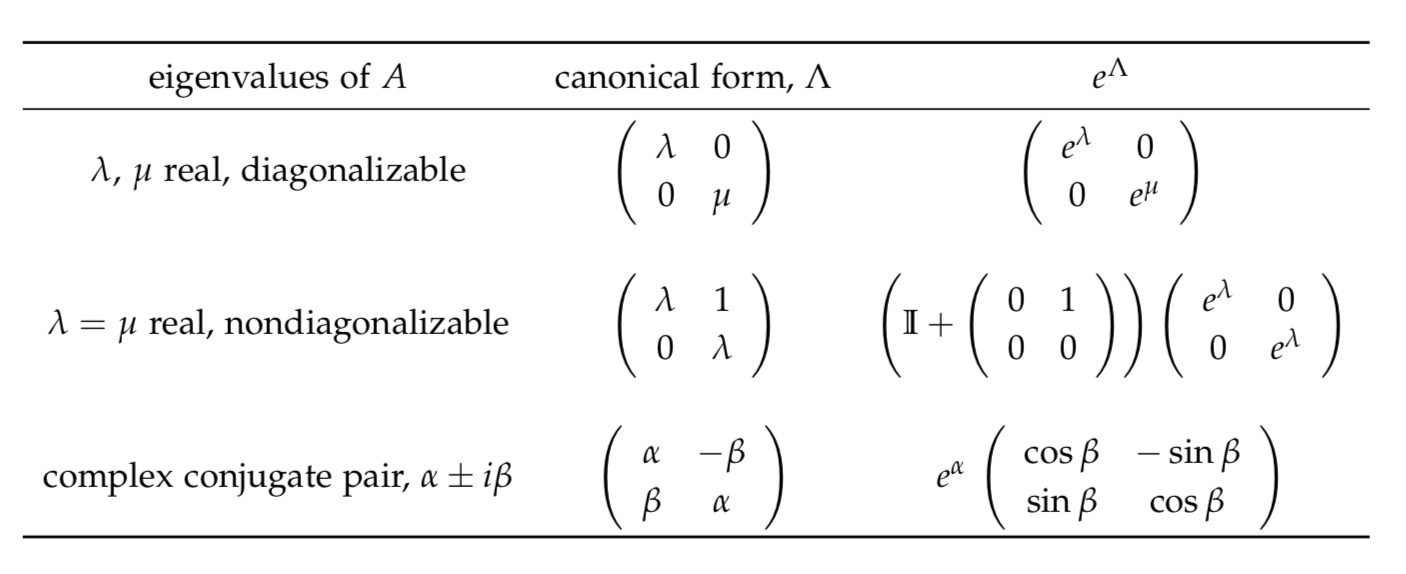
Once the transformation to \(\Lambda\) has been carried out, we will use these results to deduce \(e^{\Lambda}\).