4.8: Applications

View Nondimensionalization on YouTube

RLC Circuit

View \(RLC\) circuit on YouTube

Figure \(\PageIndex{1}\): RLC circuit diagram.

Consider a resister \(R\), an inductor \(L\), and a capacitor \(C\) connected in series as shown in Fig. \(\PageIndex{1}\). An AC generator provides a time-varying electromotive force (emf), \(\mathcal{E}(t)\), to the circuit. Here, we determine the differential equation satisfied by the charge on the capacitor.

The constitutive equations for the voltage drops across a capacitor, a resister, and an inductor are given by \[\label{eq:1}V_C=q/C,\quad V_R=iR,\quad V_L=\frac{di}{dt}L,\] where \(C\) is the capacitance, \(R\) is the resistance, and \(L\) is the inductance. The charge \(q\) and the current \(i\) are related by \[\label{eq:2}i=\frac{dq}{dt}.\]

Kirchhoff’s voltage law states that the emf \(\mathcal{E}\) applied to any closed loop is equal to the sum of the voltage drops in that loop. Applying Kirchhoff’s voltage law to the \(RLC\) circuit results in \[\label{eq:3}V_L+V_R+V_C=\mathcal{E}(t);\] or using \(\eqref{eq:1}\) and \(\eqref{eq:2}\), \[L\frac{d^2q}{dt^2}+R\frac{dq}{dt}+\frac{1}{C}q=\mathcal{E}(t).\nonumber\]

The equation for the \(RLC\) circuit is a second-order linear inhomogeneous differential equation with constant coefficients.

The AC voltage can be written as \(\mathcal{E}(t) = \mathcal{E}_0 \cos \omega t\), and the governing equation for \(q = q(t)\) can be written as \[\label{eq:4}\frac{d^2q}{dt^2}+\frac{R}{L}\frac{dq}{dt}+\frac{1}{LC}q=\frac{\mathcal{E}_0}{L}\cos\omega t.\]

Nondimensionalization of this equation will be shown to reduce the number of free parameters.

To construct dimensionless variables, we first define the natural frequency of oscillation of a system to be the frequency of oscillation in the absence of any driving or damping forces. The iconic example is the simple harmonic oscillator, with equation given by \[\overset{..}{x}+\omega_0^2x=0,\nonumber\] and general solution given by \(x(t) = A \cos \omega_0 t + B \sin\omega_0 t\). Here, the natural frequency of oscillation is \(\omega_0\), and the period of oscillation is \(T = 2π/\omega_0\). For the \(RLC\) circuit, the natural frequency of oscillation is found from the coefficient of the \(q\) term, and is given by \[\omega_0=\frac{1}{\sqrt{LC}}.\nonumber\]

Making use of \(\omega_0\), with units of one over time, we can define a dimensionless time \(\tau\) and a dimensionless charge \(Q\) by \[\tau =\omega_0t,\quad Q=\frac{\omega_0^2L}{\mathcal{E}_0}q.\nonumber\]

The resulting dimensionless equation for the \(RLC\) circuit is then given by \[\label{eq:5}\frac{d^2Q}{d\tau ^2}+\alpha\frac{dQ}{d\tau}+Q=\cos\beta\tau ,\] where \(\alpha\) and \(\beta\) are dimensionless parameters given by \[\alpha=\frac{R}{L\omega_0},\quad\beta=\frac{\omega}{\omega_0}.\nonumber\]

Notice that the original five parameters in \(\eqref{eq:4}\), namely \(R,\: L,\: C,\: \mathcal{E}_0\) and \(\omega\), have been reduced to the two dimensionless parameters \(\alpha\) and \(\beta\). We will return later to solve \(\eqref{eq:5}\) after visiting two more applications that will be shown to be governed by the same dimensionless equation.

Figure \(\PageIndex{2}\): Mass-spring system (top view).

Mass on a Spring

View Mass on a Spring on YouTube

Consider a mass connected by a spring to a fixed wall, with top view shown in Fig. \(\PageIndex{2}\). The spring force is modeled by Hooke’s law, \(F_s = −kx\), and sliding friction is modeled as \(F_f = −cdx/dt\). An external force is applied and is assumed to be sinusoidal, with \(F_e = F_0 \cos\omega t\). Newton’s equation, \(F = ma\), results in \[m\frac{d^2x}{dt^2}=-kx-c\frac{dx}{dt}+F_0\cos\omega t.\nonumber\]

Rearranging terms, we obtain \[\frac{d^2x}{dt^2}+\frac{c}{m}\frac{dx}{dt}+\frac{k}{m}x=\frac{F_0}{m}\cos\omega t.\nonumber\]

Here, the natural frequency of oscillation is given by \[\omega_0=\sqrt{\frac{k}{m}},\nonumber\] and we define a dimensionless time \(\tau\) and a dimensionless position \(X\) by \[\tau =\omega_0t,\quad X=\frac{m\omega_0^2}{F_0}x.\nonumber\]

The resulting dimensionless equation is given by \[\label{eq:6}\frac{d^2X}{d\tau ^2}+\alpha\frac{dX}{d\tau }+X=\cos\beta\tau, \] where here, \(\alpha\) and \(\beta\) are dimensionless parameters given by \[\alpha=\frac{c}{m\omega_0},\quad\beta =\frac{\omega}{\omega_0}.\nonumber\]

Notice that even though the physical problem is different, and the dimensionless variables are defined differently, the resulting dimensionless equation \(\eqref{eq:6}\) for the mass-spring system is the same as that for the \(RLC\) circuit \(\eqref{eq:5}\).

Figure \(\PageIndex{3}\): The pendulum.

Pendulum

View Pendulum on YouTube

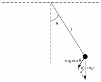
Here, we consider a mass that is attached to a massless rigid rod and is constrained to move along an arc of a circle centered at the pivot point (see Fig. \(\PageIndex{3}\)). Suppose \(l\) is the fixed length of the connecting rod, and \(θ\) is the angle it makes with the vertical.

We can apply Newton’s equation, \(F = ma\), to the mass with origin at the bottom and axis along the arc with positive direction to the right. The position \(s\) of the mass along the arc is given by \(s = lθ\). The relevant gravitational force on the pendulum is the component along the arc, and from Fig. \(\PageIndex{3}\) is observed to be \[F_g=-mg\sin\theta.\nonumber\]

We model friction to be proportional to the velocity of the pendulum along the arc, that is \[F-f=-c\overset{.}{s}=-cl\overset{.}{\theta}.\nonumber\]

With a sinusoidal external force, \(F_e = F_0 \cos\omega t\), Newton’s equation \(m\overset{..}{s}= F_g + F_f + F_e\) results in \[ml\overset{..}{\theta}=-mg\sin\theta -cl\overset{.}{\theta}+F_0\cos\omega t.\nonumber\]

Rewriting, we have \[\overset{..}{\theta}+\frac{c}{m}\overset{.}{\theta}+\frac{g}{l}\sin\theta=\frac{F_0}{ml}\cos\omega t.\nonumber\]

At small amplitudes of oscillation, we can approximate \(\sin θ\approx θ\), and the natural frequency of oscillation \(\omega_0\) of the mass is given by \[\omega_0=\sqrt{\frac{g}{l}}.\nonumber\]

Nondimensionalizing time as \(\tau = \omega_0t\), the dimensionless pendulum equation becomes \[\frac{d^2\theta}{d\tau ^2}+\alpha\frac{d\theta}{d\tau}+\sin\theta=\gamma\cos\beta\tau ,\nonumber\] where \(\alpha\), \(\beta\), and \(\gamma\) are dimensionless parameters given by \[\alpha=\frac{c}{m\omega_0},\quad\beta=\frac{\omega}{\omega_0},\quad\gamma=\frac{F_0}{ml\omega_0^2}.\nonumber\]

The nonlinearity of the pendulum equation, with the term \(\sin \theta\), results in the additional dimensionless parameter \(\gamma\). For small amplitude of oscillation, however, we can scale \(\theta\) by \(\theta =\gamma\Theta\), and the small amplitude dimensionless equation becomes \[\label{eq:7}\frac{d^2\Theta}{d\tau ^2}+\alpha\frac{d\Theta}{d\tau}+\Theta=\cos\beta\tau ,\] the same equation as \(\eqref{eq:5}\) and \(\eqref{eq:6}\).