6.1: Ordinary Points

If \(x_0\) is an ordinary point of (6.1), then it is possible to determine two power series (i.e., Taylor series) solutions for \(y = y(x)\) centered at \(x = x_0\). We illustrate the method of solution by solving two examples, with \(x_0 = 0\).

Example \(\PageIndex{1}\)

Find the general solution of \(y''+y=0\).

Solution

View tutorial on YouTube

By now, you should know that the general solution is \(y(x) = a_0 \cos x + a_1 \sin x\), with \(a_0\) and \(a_1\) constants. To find a power series solution about the point \(x_0 = 0\), we write \[y(x)=\sum\limits_{n=0}^{\infty}a_nx^n;\nonumber\] and upon differentiating term-by-term \[y'(x)=\sum\limits_{n=1}^{\infty}na_nx^{n-1},\nonumber\] and \[y''(x)=\sum\limits_{n=2}^{\infty}n(n-1)a_nx^{n-2}.\nonumber\]

Substituting the power series for \(y\) and its derivatives into the differential equation to be solved, we obtain \[\label{eq:1}\sum\limits_{n=2}^{\infty}n(n-1)a_nx^{n-2}+\sum\limits_{n=0}^{\infty}a_nx^n=0.\]

The power-series solution method requires combining the two sums on the left-hand-side of \(\eqref{eq:1}\) into a single power series in \(x\). To shift the exponent of \(x^{n−2}\) in the first sum upward by two to obtain \(x^n\), we need to shift the summation index downward by two; that is, \[\sum\limits_{n=2}^{\infty}n(n-1)a_nx^{n-2}=\sum\limits_{n=0}^{\infty}(n+2)(n+1)a_{n+2}x^n.\nonumber\]

We can then combine the two sums in \(\eqref{eq:1}\) to obtain \[\label{eq:2}\sum\limits_{n=0}^{\infty}\left((n+2)(n+1)a_{n+2}+a_n\right)x^n=0.\]

For \(\eqref{eq:2}\) to be satisfied, the coefficient of each power of \(x\) must vanish separately. (This can be proved by setting \(x = 0\) after successive differentiation.) We therefore obtain the recurrence relation \[a_{n+2}=-\frac{a_n}{(n+2)(n+1)},\quad n=0,1,2,\ldots\nonumber\]

We observe that even and odd coefficients decouple. We thus obtain two independent sequences starting with first term \(a_0\) or \(a_1\). Developing these sequences, we have for the sequence beginning with \(a_0\):

\[\begin{aligned}a_0&, \\ a_2&=-\frac{1}{2}a_0, \\ a_4&=-\frac{1}{4\cdot 3}a_2=\frac{1}{4\cdot 3\cdot 2}a_0, \\ a_6&=-\frac{1}{6\cdot 5}a_4=-\frac{1}{6!}a_0;\end{aligned}\] and the general coefficient in this sequence for \(n = 0, 1, 2,\ldots\) is \[a_{2n}=\frac{(-1)^n}{(2n)!}a_0.\nonumber\]

Also, for the sequence beginning with \(a_1\):

\[\begin{aligned}a_1&, \\ a_3&=-\frac{1}{3\cdot 2}a_1, \\ a_5&=-\frac{1}{5\cdot 4}a_3=\frac{1}{5\cdot 4\cdot 3\cdot 2}a_1, \\ a_7&=-\frac{1}{7\cdot 6}a_5=-\frac{1}{7!}a_1;\end{aligned}\] and the general coefficient in this sequence for \(n = 0, 1, 2,\ldots\) is \[a_{2n+1}=\frac{(-1)^n}{(2n+1)!}a_1.\nonumber\]

Using the principle of superposition, the general solution is therefore \[\begin{aligned}y(x)&=a_0\sum\limits_{n=0}^\infty\frac{(-1)^n}{(2n)!}x^{2n}+a_1\sum\limits_{n=0}^\infty\frac{(-1)^n}{(2n+1)!}x^{2n+1} \\ &=a_0\left(1-\frac{x^2}{2!}+\frac{x^4}{4!}-\cdots\right)+a_1\left(x-\frac{x^3}{3!}+\frac{x^5}{5!}-\cdots\right) \\ &=a_0\cos x+a_1\sin x,\end{aligned}\] as expected.

In our next example, we will solve the Airy’s Equation. This differential equation arises in the study of optics, fluid mechanics, and quantum mechanics.

Example \(\PageIndex{2}\): Airy’s Equation

Find the general solution of \(y''-xy=0\).

Solution

View tutorial on YouTube

With \[y(x)=\sum\limits_{n=0}^\infty a_nx^n,\nonumber\] the differential equation becomes \[\label{eq:3}\sum\limits_{n=2}^\infty n(n-1)a_nx^{n-2}-\sum\limits_{n=0}^\infty a_nx^{n+1}=0.\]

We shift the first sum to \(x^{n+1}\) by shifting the exponent up by three, i.e., \[\sum\limits_{n=2}^\infty n(n-1)a_nx^{n-2}=\sum\limits_{n=-1}^\infty (n+3)(n+2)a_{n+3}x^{n+1}.\nonumber\]

When combining the two sums in \(\eqref{eq:3}\), we separate out the extra \(n = −1\) term in the first sum given by \(2a_2\). Therefore, \(\eqref{eq:3}\) becomes \[\label{eq:4}2a_2+\sum\limits_{n=0}^\infty\left((n+3)(n+2)a_{n+3}-a_n\right)x^{n+1}=0.\]

Setting coefficients of powers of \(x\) to zero, we first find \(a_2 = 0\), and then obtain the recursion relation \[\label{eq:5}a_{n+3}=\frac{1}{(n+3)(n+2)}a_n.\]

Three sequences of coefficients—those starting with either \(a_0,\: a_1\) or \(a_2\)—decouple. In particular the three sequences are \[\begin{array}{l}a_0,a_3,a_6,a_9,\ldots ; \\ a_1,a_4,a_7,a_{10},\ldots ; \\ a_2,a_5,a_8,a_{11}\ldots\end{array}\nonumber\]

Since \(a_2 = 0\), we find immediately for the last sequence \[a_2=a_5=a_8=a_{11}=\cdots =0.\nonumber\]

We compute the first four nonzero terms in the power series with coefficients corresponding to the first two sequences. Starting with \(a_0\), we have \[\begin{aligned}a_0&, \\ a_3&=\frac{1}{3\cdot 2}a_0, \\ a_6&=\frac{1}{6\cdot 5\cdot 3\cdot 2}a_0, \\ a_9&=\frac{1}{9\cdot 8\cdot 6\cdot 5\cdot 3\cdot 2}a_0;\end{aligned}\] and starting with \(a_1\), \[\begin{aligned}a_1&, \\ a_4&=\frac{1}{4\cdot 3}a_1, \\ a_7&=\frac{1}{7\cdot 6\cdot 4\cdot 3}a_1, \\ a_{10}&=\frac{1}{10\cdot 9\cdot 7\cdot 6\cdot 4\cdot 3}a_1.\end{aligned}\]

The general solution for \(y = y(x)\), can therefore be written as \[\begin{aligned}y(x)&=a_0\left(1+\frac{x^3}{6}+\frac{x^6}{180}+\frac{x^9}{12960}+\cdot\right) +a_1\left(x+\frac{x^4}{12}+\frac{x^7}{504}+\frac{x^{10}}{45360}+\cdot\right) \\ &=a_0y_0(x)+a_1y_1(x).\end{aligned}\]

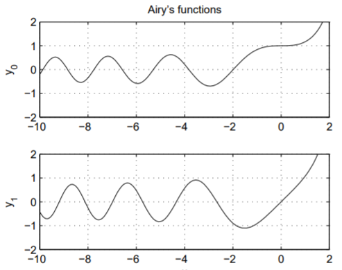
Suppose we would like to graph the solutions \(y = y_0(x)\) and \(y = y_1(x)\) versus \(x\) by solving the differential equation \(y'' − xy = 0\) numerically. What initial conditions should we use? Clearly, \(y = y_0(x)\) solves the ode with initial values \(y(0) = 1\) and \(y' (0) = 0\), while \(y = y_1(x)\) solves the ode with initial values \(y(0) = 0\) and \(y' (0) = 1\).

The numerical solutions, obtained using MATLAB, are shown in Fig. \(\PageIndex{1}\). Note that the solutions oscillate for negative \(x\) and grow exponentially for positive \(x\). This can be understood by recalling that \(y''+ y = 0\) has oscillatory sine and cosine solutions and \(y'' − y = 0\) has exponential hyperbolic sine and cosine solutions.

Figure \(\PageIndex{1}\): Numerical solution of Airy's equation.