9.1: Derivation of the Diffusion Equation

Last updated
Save as PDF

Page ID: 90432

\( \newcommand{\vecs}[1]{\overset { \scriptstyle \rightharpoonup} {\mathbf{#1}} } \) \( \newcommand{\vecd}[1]{\overset{-\!-\!\rightharpoonup}{\vphantom{a}\smash {#1}}} \)\(\newcommand{\id}{\mathrm{id}}\) \( \newcommand{\Span}{\mathrm{span}}\) \( \newcommand{\kernel}{\mathrm{null}\,}\) \( \newcommand{\range}{\mathrm{range}\,}\) \( \newcommand{\RealPart}{\mathrm{Re}}\) \( \newcommand{\ImaginaryPart}{\mathrm{Im}}\) \( \newcommand{\Argument}{\mathrm{Arg}}\) \( \newcommand{\norm}[1]{\| #1 \|}\) \( \newcommand{\inner}[2]{\langle #1, #2 \rangle}\) \( \newcommand{\Span}{\mathrm{span}}\) \(\newcommand{\id}{\mathrm{id}}\) \( \newcommand{\Span}{\mathrm{span}}\) \( \newcommand{\kernel}{\mathrm{null}\,}\) \( \newcommand{\range}{\mathrm{range}\,}\) \( \newcommand{\RealPart}{\mathrm{Re}}\) \( \newcommand{\ImaginaryPart}{\mathrm{Im}}\) \( \newcommand{\Argument}{\mathrm{Arg}}\) \( \newcommand{\norm}[1]{\| #1 \|}\) \( \newcommand{\inner}[2]{\langle #1, #2 \rangle}\) \( \newcommand{\Span}{\mathrm{span}}\)\(\newcommand{\AA}{\unicode[.8,0]{x212B}}\)

To derive the diffusion equation in one spacial dimension, we imagine a still liquid in a long pipe of constant cross sectional area. A small quantity of dye is placed in a cross section of the pipe and allowed to diffuse up and down the pipe. The dye diffuses from regions of higher concentration to regions of lower concentration.

We define \(u(x, t)\) to be the concentration of the dye at position \(x\) along the pipe, and we wish to find the pde satisfied by \(u\). It is useful to keep track of the units of the various quantities involved in the derivation and we introduce the bracket notation \([X]\) to mean the units of \(X\). Relevant dimensional units used in the derivation of the diffusion equation are mass \(m\), length \(l\), and time \(t\). Assuming that the dye concentration is uniform in every cross section of the pipe, the dimensions of concentration used here are \([u] = m/l\).

The mass of dye in the infinitesimal pipe volume located between position \(x_1\) and position \(x_2\) at time \(t\), with \(x_1 < x < x_2\), is given to order \(\Delta x = x_2 − x_1\) by \[M=u(x,t)\Delta x.\nonumber\]

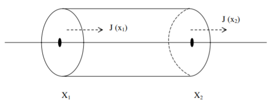
The mass of dye in this infinitesimal pipe volume changes by diffusion into and out of the cross sectional ends situated at position \(x_1\) and \(x_2\) (Figure \(\PageIndex{1}\)). We assume the rate of diffusion is proportional to the concentration gradient, a relationship known as Fick’s law of diffusion. Fick’s law of diffusion assumes the mass flux \(J\), with units \([J] = m/t\) across a cross section of the pipe is given by \[\label{eq:1}J=-Du_x,\] where the diffusion constant \(D > 0\) has units \([D] = l^2/t\), and we have used the notation \(u_x = \partial u/\partial x\). The mass flux is opposite in sign to the gradient of concentration so that the flux is from high concentration to low concentration. The time rate of change in the mass of dye between \(x_1\) and \(x_2\) is given by the difference between the mass flux into and the mass flux out of the infinitesimal cross sectional

Figure \(\PageIndex{1}\): Derivation of the diffusion equation.

volume. A positive mass flux signifies diffusion from left to right. Therefore, the time rate of change of the dye mass is given by \[\frac{dM}{dt}=J(x_1, t)-J(x_2, t),\nonumber\] or rewriting in terms of \(u(x,t)\):

\[u_t(x,t)\Delta x=D(u_x(x_2,t)-u_x(x_1,t)).\nonumber\]

Dividing by \(\Delta x\) and taking the limit \(\Delta x\to 0\) results in the diffusion equation:

\[u_t=Du_{xx}.\nonumber\]

We note that the diffusion equation is identical to the heat conduction equation, where \(u\) is temperature, and the constant \(D\) (commonly written as \(\kappa\)) is the thermal conductivity.