9.2: Derivation of the Wave Equation

Last updated
Save as PDF

Page ID: 90433

\( \newcommand{\vecs}[1]{\overset { \scriptstyle \rightharpoonup} {\mathbf{#1}} } \) \( \newcommand{\vecd}[1]{\overset{-\!-\!\rightharpoonup}{\vphantom{a}\smash {#1}}} \)\(\newcommand{\id}{\mathrm{id}}\) \( \newcommand{\Span}{\mathrm{span}}\) \( \newcommand{\kernel}{\mathrm{null}\,}\) \( \newcommand{\range}{\mathrm{range}\,}\) \( \newcommand{\RealPart}{\mathrm{Re}}\) \( \newcommand{\ImaginaryPart}{\mathrm{Im}}\) \( \newcommand{\Argument}{\mathrm{Arg}}\) \( \newcommand{\norm}[1]{\| #1 \|}\) \( \newcommand{\inner}[2]{\langle #1, #2 \rangle}\) \( \newcommand{\Span}{\mathrm{span}}\) \(\newcommand{\id}{\mathrm{id}}\) \( \newcommand{\Span}{\mathrm{span}}\) \( \newcommand{\kernel}{\mathrm{null}\,}\) \( \newcommand{\range}{\mathrm{range}\,}\) \( \newcommand{\RealPart}{\mathrm{Re}}\) \( \newcommand{\ImaginaryPart}{\mathrm{Im}}\) \( \newcommand{\Argument}{\mathrm{Arg}}\) \( \newcommand{\norm}[1]{\| #1 \|}\) \( \newcommand{\inner}[2]{\langle #1, #2 \rangle}\) \( \newcommand{\Span}{\mathrm{span}}\)\(\newcommand{\AA}{\unicode[.8,0]{x212B}}\)

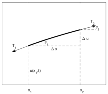
To derive the wave equation in one spacial dimension, we imagine an elastic string that undergoes small amplitude transverse vibrations. We define \(u(x, t)\) to be the vertical displacement of the string from the \(x\)-axis at position \(x\) and time \(t\), and we wish to find the pde satisfied by \(u\). We define \(\rho\) to be the constant mass density of the string, \(T\) the tension of the string, and \(\theta\) the angle between the string and the horizontal line. We consider an infinitesimal string element located between \(x_1\) and \(x_2\), with \(\Delta x = x_2 − x_1\), as shown in Fig. \(\PageIndex{1}\). The governing equations are Newton’s law of motion for the horizontal and vertical acceleration of our infinitesimal string element, and we assume that the string element only accelerates vertically. Therefore, the horizontal forces must balance and we have \[T_2\cos\theta_2=T_1\cos\theta_1.\nonumber\]

The vertical forces result in a vertical acceleration, and with \(u_{tt}\) the vertical acceleration of the string element and \(\rho\sqrt{\Delta x^2+\Delta u^2}=\rho\Delta x\sqrt{1+u_x^2}\) its mass, where we have used \(u_x = \Delta u/\Delta x\), exact as \(\Delta x\to 0\), we have \[\rho\Delta x\sqrt{1+u_x^2}u_{tt}=T_2\sin\theta_2-T_1\sin\theta_1.\nonumber\]

Figure \(\PageIndex{1}\): Derivation of the wave equation.

We now make the assumption of small vibrations, that is \(\Delta u ≪ \Delta x\), or equivalently \(u_x ≪ 1\). Note that \([u] = l\) so that \(u_x\) is dimensionless. With this approximation, to leading-order in \(u_x\) we have \[\cos\theta_2=\cos\theta_1=1,\nonumber\] \[\sin\theta_2=u_x(x_2,t),\quad\sin\theta_1=u_x(x_1,t),\nonumber\] and \[\sqrt{1+u_x^2}=1.\nonumber\]

Therefore, to leading order \(T_1 = T_2 = T\), (i.e., the tension in the string is approximately constant), and \[\rho\Delta xu_{tt}=T(u_x(x_2,t)-u_x(x_1,t)).\nonumber\]

Dividing by \(\Delta x\) and taking the limit \(\Delta x\to 0\) results in the wave equation \[u_{tt}=c^2u_{xx},\nonumber\] where \(c^2=T/\rho\). Since \([T]=ml/t^2\) and \([\rho]=m/l\), we have \([c^2]=l^2/t^2\) so that \(c\) has units of velocity.