Mathematics LibreTexts

3.5: Two dimensional systems and their vector fields

  • Page ID
    366
  • \( \newcommand{\vecs}[1]{\overset { \scriptstyle \rightharpoonup} {\mathbf{#1}} } \)

    \( \newcommand{\vecd}[1]{\overset{-\!-\!\rightharpoonup}{\vphantom{a}\smash {#1}}} \)

    \( \newcommand{\id}{\mathrm{id}}\) \( \newcommand{\Span}{\mathrm{span}}\)

    ( \newcommand{\kernel}{\mathrm{null}\,}\) \( \newcommand{\range}{\mathrm{range}\,}\)

    \( \newcommand{\RealPart}{\mathrm{Re}}\) \( \newcommand{\ImaginaryPart}{\mathrm{Im}}\)

    \( \newcommand{\Argument}{\mathrm{Arg}}\) \( \newcommand{\norm}[1]{\| #1 \|}\)

    \( \newcommand{\inner}[2]{\langle #1, #2 \rangle}\)

    \( \newcommand{\Span}{\mathrm{span}}\)

    \( \newcommand{\id}{\mathrm{id}}\)

    \( \newcommand{\Span}{\mathrm{span}}\)

    \( \newcommand{\kernel}{\mathrm{null}\,}\)

    \( \newcommand{\range}{\mathrm{range}\,}\)

    \( \newcommand{\RealPart}{\mathrm{Re}}\)

    \( \newcommand{\ImaginaryPart}{\mathrm{Im}}\)

    \( \newcommand{\Argument}{\mathrm{Arg}}\)

    \( \newcommand{\norm}[1]{\| #1 \|}\)

    \( \newcommand{\inner}[2]{\langle #1, #2 \rangle}\)

    \( \newcommand{\Span}{\mathrm{span}}\) \( \newcommand{\AA}{\unicode[.8,0]{x212B}}\)

    \( \newcommand{\vectorA}[1]{\vec{#1}}      % arrow\)

    \( \newcommand{\vectorAt}[1]{\vec{\text{#1}}}      % arrow\)

    \( \newcommand{\vectorB}[1]{\overset { \scriptstyle \rightharpoonup} {\mathbf{#1}} } \)

    \( \newcommand{\vectorC}[1]{\textbf{#1}} \)

    \( \newcommand{\vectorD}[1]{\overrightarrow{#1}} \)

    \( \newcommand{\vectorDt}[1]{\overrightarrow{\text{#1}}} \)

    \( \newcommand{\vectE}[1]{\overset{-\!-\!\rightharpoonup}{\vphantom{a}\smash{\mathbf {#1}}}} \)

    \( \newcommand{\vecs}[1]{\overset { \scriptstyle \rightharpoonup} {\mathbf{#1}} } \)

    \( \newcommand{\vecd}[1]{\overset{-\!-\!\rightharpoonup}{\vphantom{a}\smash {#1}}} \)

    \(\newcommand{\avec}{\mathbf a}\) \(\newcommand{\bvec}{\mathbf b}\) \(\newcommand{\cvec}{\mathbf c}\) \(\newcommand{\dvec}{\mathbf d}\) \(\newcommand{\dtil}{\widetilde{\mathbf d}}\) \(\newcommand{\evec}{\mathbf e}\) \(\newcommand{\fvec}{\mathbf f}\) \(\newcommand{\nvec}{\mathbf n}\) \(\newcommand{\pvec}{\mathbf p}\) \(\newcommand{\qvec}{\mathbf q}\) \(\newcommand{\svec}{\mathbf s}\) \(\newcommand{\tvec}{\mathbf t}\) \(\newcommand{\uvec}{\mathbf u}\) \(\newcommand{\vvec}{\mathbf v}\) \(\newcommand{\wvec}{\mathbf w}\) \(\newcommand{\xvec}{\mathbf x}\) \(\newcommand{\yvec}{\mathbf y}\) \(\newcommand{\zvec}{\mathbf z}\) \(\newcommand{\rvec}{\mathbf r}\) \(\newcommand{\mvec}{\mathbf m}\) \(\newcommand{\zerovec}{\mathbf 0}\) \(\newcommand{\onevec}{\mathbf 1}\) \(\newcommand{\real}{\mathbb R}\) \(\newcommand{\twovec}[2]{\left[\begin{array}{r}#1 \\ #2 \end{array}\right]}\) \(\newcommand{\ctwovec}[2]{\left[\begin{array}{c}#1 \\ #2 \end{array}\right]}\) \(\newcommand{\threevec}[3]{\left[\begin{array}{r}#1 \\ #2 \\ #3 \end{array}\right]}\) \(\newcommand{\cthreevec}[3]{\left[\begin{array}{c}#1 \\ #2 \\ #3 \end{array}\right]}\) \(\newcommand{\fourvec}[4]{\left[\begin{array}{r}#1 \\ #2 \\ #3 \\ #4 \end{array}\right]}\) \(\newcommand{\cfourvec}[4]{\left[\begin{array}{c}#1 \\ #2 \\ #3 \\ #4 \end{array}\right]}\) \(\newcommand{\fivevec}[5]{\left[\begin{array}{r}#1 \\ #2 \\ #3 \\ #4 \\ #5 \\ \end{array}\right]}\) \(\newcommand{\cfivevec}[5]{\left[\begin{array}{c}#1 \\ #2 \\ #3 \\ #4 \\ #5 \\ \end{array}\right]}\) \(\newcommand{\mattwo}[4]{\left[\begin{array}{rr}#1 \amp #2 \\ #3 \amp #4 \\ \end{array}\right]}\) \(\newcommand{\laspan}[1]{\text{Span}\{#1\}}\) \(\newcommand{\bcal}{\cal B}\) \(\newcommand{\ccal}{\cal C}\) \(\newcommand{\scal}{\cal S}\) \(\newcommand{\wcal}{\cal W}\) \(\newcommand{\ecal}{\cal E}\) \(\newcommand{\coords}[2]{\left\{#1\right\}_{#2}}\) \(\newcommand{\gray}[1]{\color{gray}{#1}}\) \(\newcommand{\lgray}[1]{\color{lightgray}{#1}}\) \(\newcommand{\rank}{\operatorname{rank}}\) \(\newcommand{\row}{\text{Row}}\) \(\newcommand{\col}{\text{Col}}\) \(\renewcommand{\row}{\text{Row}}\) \(\newcommand{\nul}{\text{Nul}}\) \(\newcommand{\var}{\text{Var}}\) \(\newcommand{\corr}{\text{corr}}\) \(\newcommand{\len}[1]{\left|#1\right|}\) \(\newcommand{\bbar}{\overline{\bvec}}\) \(\newcommand{\bhat}{\widehat{\bvec}}\) \(\newcommand{\bperp}{\bvec^\perp}\) \(\newcommand{\xhat}{\widehat{\xvec}}\) \(\newcommand{\vhat}{\widehat{\vvec}}\) \(\newcommand{\uhat}{\widehat{\uvec}}\) \(\newcommand{\what}{\widehat{\wvec}}\) \(\newcommand{\Sighat}{\widehat{\Sigma}}\) \(\newcommand{\lt}{<}\) \(\newcommand{\gt}{>}\) \(\newcommand{\amp}{&}\) \(\definecolor{fillinmathshade}{gray}{0.9}\)

    Let us take a moment to talk about constant coefficient linear homogeneous systems in the plane. Much intuition can be obtained by studying this simple case. Suppose we use coordinates \((x,y)\) for the plane as usual, and suppose \(P=\left[\begin{array}{cc}{a}&{b}\\{c}&{d}\end{array}\right]\) is a \(2\, \times \, 2\) matrix . Consider the system

    \[\label{pln:eq} \begin{bmatrix} x \\ y \end{bmatrix} ' = P \begin{bmatrix} x \\ y \end{bmatrix} \qquad \text{or} \qquad \begin{bmatrix} x \\ y \end{bmatrix} ' = \begin{bmatrix} a & b \\ c & d \end{bmatrix} \begin{bmatrix} x \\ y \end{bmatrix} . \]

    The system is autonomous (compare this section to Section 1.6) and so we can draw a vector field (see end of Section 3.1). We will be able to visually tell what the vector field looks like and how the solutions behave, once we find the eigenvalues and eigenvectors of the matrix \(P\). For this section, we assume that \(P\) has two eigenvalues and two corresponding eigenvectors.

    1

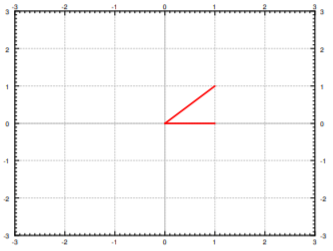
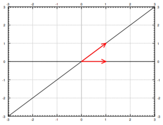
    Suppose that the eigenvalues of \(P\) are real and positive. We find two corresponding eigenvectors and plot them in the plane. For example, take the matrix \( \begin{bmatrix} 1&1 \\ 0&2 \end{bmatrix} \). The eigenvalues are 1 and 2 and corresponding eigenvectors are \( \begin{bmatrix} 1\\0 \end{bmatrix} \) and \( \begin{bmatrix} 1 \\1 \end{bmatrix} \). See Figure \(\PageIndex{1}\).

    clipboard_ec4e6a529522375995dbb822f629f9b2d.png
    Figure \(\PageIndex{1}\): Eigenvectors of \(P\).

    Now suppose that \(x\) and \(y\) are on the line determined by an eigenvector \( \vec{v} \) for an eigenvalue \( \lambda \). That is, \( \begin{bmatrix} x \\ y \end{bmatrix} = a \vec{v} \) for some scalar \(a\). Then

    \[ \begin{bmatrix} x\\y \end{bmatrix}' = P \begin{bmatrix} x\\y \end{bmatrix} = P(a \vec{v}) = a(P \vec{v}) = a \lambda \vec{v} \nonumber \]

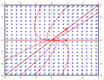
    The derivative is a multiple of \( \vec{v} \) and hence points along the line determined by \( \vec{v} \). As \( \lambda > 0 \), the derivative points in the direction of \( vec{v} \) when \(\alpha \) is positive and in the opposite direction when \( \alpha\) is negative. Let us draw the lines determined by the eigenvectors, and let us draw arrows on the lines to indicate the directions. See Figure \(\PageIndex{2}\).

    We fill in the rest of the arrows for the vector field and we also draw a few solutions. See Figure \(\PageIndex{3}\). Notice that the picture looks like a source with arrows coming out from the origin. Hence we call this type of picture a source or sometimes an unstable node.
    clipboard_ee645f5487135da1c7f2483f0da636583.png
    Figure \(\PageIndex{2}\): Eigenvectors of \(P\) with directions.
    clipboard_e528d31823d8208b0736f429a9fdb4a9c.png
    Figure \(\PageIndex{3}\): Example source vector field with eigenvectors and solutions.

    2

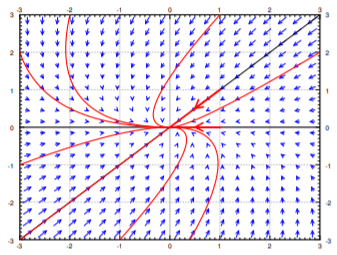
    Suppose both eigenvalues were negative. For example, take the negation of the matrix in case 1, \( \begin{bmatrix} -1 & -1\\ 0 & -2 \end{bmatrix} \). The eigenvalues are -1 and -2 and corresponding eigenvectors are the same, \( \begin{bmatrix} 1\\0 \end{bmatrix} \) and \(\begin{bmatrix}1\\1\end{bmatrix}\). The calculation and the picture are almost the same. The only difference is that the eigenvalues are negative and hence all arrows are reversed. We get the picture in Figure \(\PageIndex{4}\). We call this kind of picture a sink or sometimes a stable node.
    clipboard_e9178e6f388dc7b04e3eaa3a2be771ffd.png
    Figure \(\PageIndex{4}\): Example sink vector field with eigenvectors and solutions.

    3

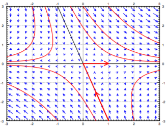
    Suppose one eigenvalue is positive and one is negative. For example the matrix \(\left[\begin{array}{cc}{1}&{1}\\{0}&{-2}\end{array}\right]\). The eigenvalues are \(1\) and \(−2\) and corresponding eigenvectors are \(\left[\begin{array}{c}{1}\\{0}\end{array}\right]\) and \(\left[\begin{array}{c}{1}\\{-3}\end{array}\right]\).

    We reverse the arrows on one line (corresponding to the negative eigenvalue) and we obtain the picture in Figure \(\PageIndex{5}\). We call this picture a saddle point.

    clipboard_e85b9be4b1aac3e5dcc457706f75b9649.png
    Figure \(\PageIndex{5}\): Example saddle vector field with eigenvectors and solutions.

    For the next three cases we will assume the eigenvalues are complex. In this case the eigenvectors are also complex and we cannot just plot them in the plane.

    4

    Suppose the eigenvalues are purely imaginary. That is, suppose the eigenvalues are \(\pm ib\). For example, let \( P = \begin{bmatrix} 0&1\\-4&0\end{bmatrix} \). The eigenvalues turn out to be \(\pm 2i \) and eigenvectors are \( \begin{bmatrix} 1 \\ 2i \end{bmatrix} \) and \(\begin{bmatrix} 1 \\ -2i \end{bmatrix} \). Consider the eigenvalue \(2i\) and its eigenvector \( \begin{bmatrix} 1\\ 2i \end{bmatrix}\). The real and imaginary parts of \(\vec{v} e^{i 2t} \) are

    \[ Re \begin{bmatrix} 1\\2i \end{bmatrix} e^{i2t} = \begin{bmatrix} cos(2t)\\-2sin(2t) \end{bmatrix},\quad Im \begin{bmatrix} 1\\2i \end{bmatrix} e^{i2t} = \begin{bmatrix} sin(2t) \\2cos(2t) \end{bmatrix} \nonumber \]

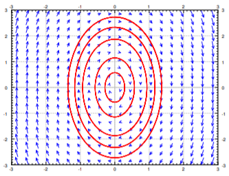
    We can take any linear combination of them to get other solutions, which one we take depends on the initial conditions. Now note that the real part is a parametric equation for an ellipse. Same with the imaginary part and in fact any linear combination of the two. This is what happens in general when the eigenvalues are purely imaginary. So when the eigenvalues are purely imaginary, we get ellipses for the solutions. This type of picture is sometimes called a center. See Figure \(\PageIndex{6}\).

    clipboard_e3900fc76c3aa811042410b8f352a9be3.png
    Figure \(\PageIndex{6}\): Example center vector field.

    5

    Now suppose the complex eigenvalues have a positive real part. That is, suppose the eigenvalues are \(a \pm ib \) for some \(a > 0 \). For example, let \(P = \begin{bmatrix} 1&1 \\ -4&1 \end{bmatrix} \). The eigenvalues turn out to be \( 1 \pm 2i \) and eigenvectors are \( \begin{bmatrix}1\\2i \end{bmatrix} \) and \( \begin{bmatrix} 1 \\ -2i \end{bmatrix}\). We take \(1\pm 2i \) and its eigenvector \( \begin{bmatrix} 1 \\ 2i \end{bmatrix} \) and find the real and imaginary of \(\vec{v}e^{(1+2i)t}\) are

    \[ Re \begin{bmatrix} 1\\2i \end{bmatrix} e^{(1+2i)t} =e^t \begin{bmatrix} cos(2t)\\-2sin(2t) \end{bmatrix} \quad Im \begin{bmatrix} 1\\2i \end{bmatrix} e^{(1+2i)t} =e^t \begin{bmatrix} sin(2t) \\2cos(2t) \end{bmatrix} \nonumber \]

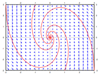
    Note the \(e^t\) in front of the solutions. This means that the solutions grow in magnitude while spinning around the origin. Hence we get a spiral source. See Figure \(\PageIndex{7}\).

    clipboard_e73c177c1987559dc1b68a18a1b052a18.png
    Figure \(\PageIndex{7}\): Example spiral source vector field.

    6

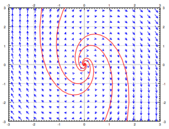
    Finally suppose the complex eigenvalues have a negative real part. That is, suppose the eigenvalues are \(-a \pm ib \) for some \( a > 0 \). For example, let \( P = \begin{bmatrix} -1& -1 \\ 4 & -1\end{bmatrix} \). The eigenvalues turn out to be \(-1 \pm 2i \) and eigenvectors are \(\begin{bmatrix} 1\\ -2i \end{bmatrix} \) and \(\begin{bmatrix} 1\\ 2i \end{bmatrix}\). We take \( -1-2i \) and its eigenvector \(\begin{bmatrix} 1\\ 2i \end{bmatrix}\) and find the real and imaginary of \(\vec{v} e^{(-1-2i)t} \) are

    \[Re \begin{bmatrix} 1\\2i \end{bmatrix} e^{(-1-2i)t} =e^{-t} \begin{bmatrix} cos(2t)\\ 2sin(2t) \end{bmatrix} \quad Im \begin{bmatrix} 1\\2i \end{bmatrix} e^{(-1-2i)t} =e^{-t} \begin{bmatrix} -sin(2t) \\2cos(2t) \end{bmatrix} \nonumber \]

    Note the \(e^{-t}\) in front of the solutions. This means that the solutions shrink in magnitude while spinning around the origin. Hence we get a spiral sink. See Figure \(\PageIndex{8}\).

    clipboard_e7753896f006d30fa4c62691dbc93958a.png
    Figure \(\PageIndex{8}\): Example spiral sink vector field.

    We summarize the behavior of linear homogeneous two dimensional systems given by a nonsingular matrix in Table \(\PageIndex{1}\). Systems where one of the eigenvalues is zero (the matrix is singular) come up in practice from time to time, see Example 3.1.2, and the pictures are somewhat different (simpler in a way). See the exercises.

    Table \(\PageIndex{1}\): Summary of behavior of linear homogeneous two dimensional systems.
    Eigenvalues Behavior
    real and both positive source / unstable node
    real and both negative sink / stable node
    real and opposite signs saddle
    purely imaginary center point / ellipses
    complex with positive real part spiral source
    complex with negative real part spiral sink

    Contributors and Attributions


    This page titled 3.5: Two dimensional systems and their vector fields is shared under a CC BY-SA 4.0 license and was authored, remixed, and/or curated by Jiří Lebl via source content that was edited to the style and standards of the LibreTexts platform.