5.2: Classical Orthogonal Polynomials

There are other basis functions that can be used to develop series representations of functions. In this section we introduce the classical orthogonal polynomials. We begin by noting that the sequence of functions \(\left\{1, x, x^{2}, \ldots\right\}\) is a basis of linearly independent functions. In fact, by the Stone-Weierstraß Approximation Theorem \(^{1}\) this set is a basis of \(L_{\sigma}^{2}(a, b)\), the space of square integrable functions over the interval \([a, b]\) relative to weight \(\sigma(x)\). However, we will show that the sequence of functions \(\left\{1, x, x^{2}, \ldots\right\}\) does not provide an orthogonal basis for these spaces. We will then proceed to find an appropriate orthogonal basis of functions.

Theorem \(\PageIndex{1}\): Stone-Weierstra\(\beta\) Approximation Theorem

Suppose \(f\) is a continuous function defined on the interval \([a, b]\). For every \(e > 0\), there exists a polynomial function \(P(x)\) such that for all \(x ∈ [a, b]\), we have \(| f(x) − P(x)| < e\). Therefore, every continuous function defined on \([a, b]\) can be uniformly approximated as closely as we wish by a polynomial function.

We are familiar with being able to expand functions over the basis \(\left\{1, x, x^{2}, \ldots\right.\) since these expansions are just Maclaurin series representations of the functions about \(x=0\), \[f(x) \sim \sum_{n=0}^{\infty} c_{n} x^{n} .\nonumber \]

However, this basis is not an orthogonal set of basis functions. One can easily see this by integrating the product of two even, or two odd, basis functions with \(\sigma(x)=1\) and \((a, b)=(-1,1)\). For example, \[\int_{-1}^{1} x^{0} x^{2} d x=\frac{2}{3} .\nonumber \]

Since we have found that orthogonal bases have been useful in determining the coefficients for expansions of given functions, we might ask, "Given a set of linearly independent basis vectors, can one find an orthogonal basis of the given space?" The answer is yes. We recall from introductory linear algebra, which mostly covers finite dimensional vector spaces, that there is a method for carrying this out called the Gram-Schmidt Orthogonalization Process. We will review this process for finite dimensional vectors and then generalize to function spaces.

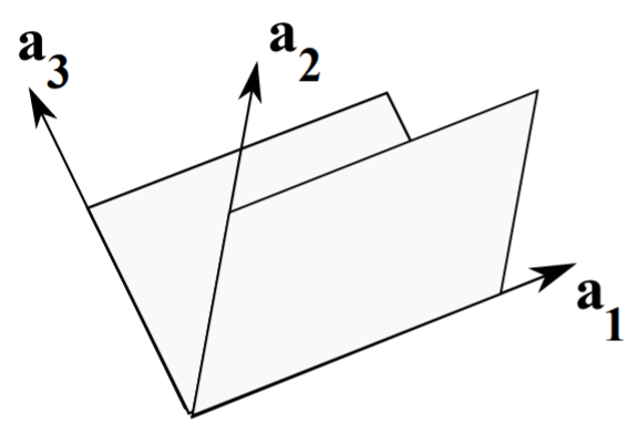
Let’s assume that we have three vectors that span the usual three dimensional space, \(\mathbf{R}^{3}\), given by \(\mathbf{a}_{1}, \mathbf{a}_{2}\), and \(\mathbf{a}_{3}\) and shown in Figure \(\PageIndex{1}\). We seek an orthogonal basis \(\mathbf{e}_{1}, \mathbf{e}_{2}\), and \(\mathbf{e}_{3}\), beginning one vector at a time.

Figure \(\PageIndex{1}\): The basis \(\mathbf{a}_{1}, \mathbf{a}_{2}\), and \(\mathbf{a}_{3}\), of \(\mathbf{R}^{3}\).

First we take one of the original basis vectors, say \(\mathbf{a}_{1}\), and define \[\mathbf{e}_{1}=\mathbf{a}_{1} .\nonumber \] It is sometimes useful to normalize these basis vectors, denoting such a normalized vector with a "hat": \[\hat{\mathbf{e}}_{1}=\frac{\mathbf{e}_{1}}{e_{1}}\nonumber \] where \(e_{1}=\sqrt{\mathbf{e}_{1} \cdot \mathbf{e}_{1}}\).

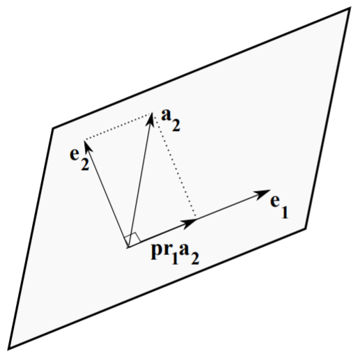
Next, we want to determine an \(\mathbf{e}_{2}\) that is orthogonal to \(\mathbf{e}_{1}\). We take another element of the original basis, \(\mathbf{a}_{2}\). In Figure \(\PageIndex{2}\) we show the orientation of the vectors. Note that the desired orthogonal vector is \(\mathbf{e}_{2}\). We can now write \(\mathbf{a}_{2}\) as the sum of \(\mathbf{e}_{2}\) and the projection of \(\mathbf{a}_{2}\) on \(\mathbf{e}_{1}\). Denoting this projection by \(\mathbf{p r}_{1} \mathbf{a}_{2}\), we then have \[\mathbf{e}_{2}=\mathbf{a}_{2}-\mathbf{p r}_{1} \mathbf{a}_{2} .\label{eq:1} \]

Figure \(\PageIndex{2}\): A plot of the vectors \(\mathbf{e}_{1}, \mathbf{a}_{2}\), and \(\mathbf{e}_{2}\) needed to find the projection of \(a_{2}\), on \(e_{1}\).

Recall the projection of one vector onto another from your vector calculus class. \[\mathbf{p r}_{1} \mathbf{a}_{2}=\frac{\mathbf{a}_{2} \cdot \mathbf{e}_{1}}{e_{1}^{2}} \mathbf{e}_{1} .\label{eq:2}\] This is easily proven by writing the projection as a vector of length \(a_{2} \cos \theta\) in direction \(\hat{\mathbf{e}}_{1}\), where \(\theta\) is the angle between \(\mathbf{e}_{1}\) and \(\mathbf{a}_{2}\). Using the definition of the dot product, \(\mathbf{a} \cdot \mathbf{b}=a b \cos \theta\), the projection formula follows.

Combining Equations \(\eqref{eq:1}\)-\(\eqref{eq:2}\), we find that \[\mathbf{e}_{2}=\mathbf{a}_{2}-\frac{\mathbf{a}_{2} \cdot \mathbf{e}_{1}}{e_{1}^{2}} \mathbf{e}_{1} .\label{eq:3}\] It is a simple matter to verify that \(\mathbf{e}_{2}\) is orthogonal to \(\mathbf{e}_{1}\) : \[\begin{align} \mathbf{e}_{2} \cdot \mathbf{e}_{1} &=\mathbf{a}_{2} \cdot \mathbf{e}_{1}-\frac{\mathbf{a}_{2} \cdot \mathbf{e}_{1}}{e_{1}^{2}} \mathbf{e}_{1} \cdot \mathbf{e}_{1}\nonumber \\ &=\mathbf{a}_{2} \cdot \mathbf{e}_{1}-\mathbf{a}_{2} \cdot \mathbf{e}_{1}=0 .\label{eq:4} \end{align}\]

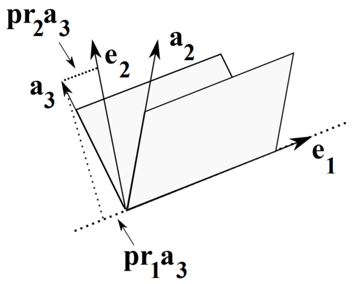
Next, we seek a third vector \(\mathbf{e}_{3}\) that is orthogonal to both \(\mathbf{e}_{1}\) and \(\mathbf{e}_{2}\). Pictorially, we can write the given vector \(\mathbf{a}_{3}\) as a combination of vector projections along \(\mathbf{e}_{1}\) and \(\mathbf{e}_{2}\) with the new vector. This is shown in Figure \(\PageIndex{3}\). Thus, we can see that \[\mathbf{e}_{3}=\mathbf{a}_{3}-\frac{\mathbf{a}_{3} \cdot \mathbf{e}_{1}}{e_{1}^{2}} \mathbf{e}_{1}-\frac{\mathbf{a}_{3} \cdot \mathbf{e}_{2}}{e_{2}^{2}} \mathbf{e}_{2} .\label{eq:5}\] Again, it is a simple matter to compute the scalar products with \(\mathbf{e}_{1}\) and \(\mathbf{e}_{2}\) to verify orthogonality.

Figure \(\PageIndex{3}\): A plot of vectors for determining \(\mathbf{e}_3\).

We can easily generalize this procedure to the \(N\)-dimensional case. Let \(\mathbf{a}_{n}, n=1, \ldots, N\) be a set of linearly independent vectors in \(\mathbf{R}^{N}\). Then, an orthogonal basis can be found by setting \(\mathbf{e}_{1}=\mathbf{a}_{1}\) and defining \[\mathbf{e}_{n}=\mathbf{a}_{n}-\sum_{j=1}^{n-1} \frac{\mathbf{a}_{n} \cdot \mathbf{e}_{j}}{e_{j}^{2}} \mathbf{e}_{j}, \quad n=2,3, \ldots, N\label{eq:6}\]

Now, we can generalize this idea to (real) function spaces. Let \(f_{n}(x)\), \(n \in N_{0}=\{0,1,2, \ldots\}\), be a linearly independent sequence of continuous functions defined for \(x \in[a, b]\). Then, an orthogonal basis of functions, \(\phi_{n}(x), n \in N_{0}\) can be found and is given by \[\phi_{0}(x)=f_{0}(x)\nonumber \] and \[\phi_{n}(x)=f_{n}(x)-\sum_{j=0}^{n-1} \frac{\left\langle f_{n}, \phi_{j}\right\rangle}{\left\|\phi_{j}\right\|^{2}} \phi_{j}(x), \quad n=1,2, \ldots .\label{eq:7}\]

Here we are using inner products relative to weight \(\sigma(x)\), \[\langle f, g\rangle=\int_{a}^{b} f(x) g(x) \sigma(x) d x .\label{eq:8}\] Note the similarity between the orthogonal basis in \(\eqref{eq:7}\) and the expression for the finite dimensional case in Equation \(\eqref{eq:6}\).

Example \(\PageIndex{1}\)

Apply the Gram-Schmidt Orthogonalization process to the set \(f_{n}(x)=\) \(x^{n}, n \in N_{0}\), when \(x \in(-1,1)\) and \(\sigma(x)=1\).

Solution

First, we have \(\phi_{0}(x)=f_{0}(x)=1\). Note that \[\int_{-1}^{1} \phi_{0}^{2}(x) d x=2 .\nonumber \] We could use this result to fix the normalization of the new basis, but we will hold off doing that for now.

Now, we compute the second basis element: \[\begin{align} \phi_{1}(x) &=f_{1}(x)-\frac{\left\langle f_{1}, \phi_{0}\right\rangle}{\left\|\phi_{0}\right\|^{2}} \phi_{0}(x)\nonumber \\ &=x-\frac{\langle x, 1\rangle}{\|1\|^{2}} 1=x,\label{eq:9} \end{align}\] since \(\langle x, 1\rangle\) is the integral of an odd function over a symmetric interval.

For \(\phi_{2}(x)\), we have \[\begin{align} \phi_{2}(x) &=f_{2}(x)-\frac{\left\langle f_{2}, \phi_{0}\right\rangle}{\left\|\phi_{0}\right\|^{2}} \phi_{0}(x)-\frac{\left\langle f_{2}, \phi_{1}\right\rangle}{\left\|\phi_{1}\right\|^{2}} \phi_{1}(x)\nonumber \\ &=x^{2}-\frac{\left\langle x^{2}, 1\right\rangle}{\|1\|^{2}} 1-\frac{\left\langle x^{2}, x\right\rangle}{\|x\|^{2}} x\nonumber \\ &=x^{2}-\frac{\int_{-1}^{1} x^{2} d x}{\int_{-1}^{1} d x}\nonumber \\ &=x^{2}-\frac{1}{3}\label{eq:10} \end{align}\]

So far, we have the orthogonal set \(\left\{1, x, x^{2}-\frac{1}{3}\right\}\). If one chooses to normalize these by forcing \(\phi_{n}(1)=1\), then one obtains the classical Legendre polynomials, \(P_{n}(x)\). Thus, \[P_{2}(x)=\frac{1}{2}\left(3 x^{2}-1\right) .\nonumber \] Note that this normalization is different than the usual one. In fact, we see the \(P_{2}(x)\) does not have a unit norm, \[\left\|P_{2}\right\|^{2}=\int_{-1}^{1} P_{2}^{2}(x) d x=\frac{2}{5} .\nonumber \]

The set of Legendre\(^{2}\) polynomials is just one set of classical orthogonal polynomials that can be obtained in this way. Many of these special functions had originally appeared as solutions of important boundary value problems in physics. They all have similar properties and we will just elaborate some of these for the Legendre functions in the next section. Others in this group are shown in Table \(\PageIndex{1}\).

Note

Adrien-Marie Legendre (1752-1833) was a French mathematician who made many contributions to analysis and algebra.

Table \(\PageIndex{1}\): Common classical orthogonal polynomials with the interval and weight function used to define them.

Polynomial	Symbol	Interval	\(\sigma(x)\)
Hermite	\(H_{n}(x)\)	\((-\infty, \infty)\)	\(e^{-x^{2}}\)
Laguerre	\(L_{n}^{\alpha}(x)\)	\([0, \infty)\)	\(e^{-x}\)
Legendre	\(P_{n}(x)\)	\((-1,1)\)	1
Gegenbauer	\(C_{n}^{\lambda}(x)\)	\((-1,1)\)	\(\left(1-x^{2}\right)^{\lambda-1 / 2}\)
Tchebychef of the 1st kind	\(T_{n}(x)\)	\((-1,1)\)	\(\left(1-x^{2}\right)^{-1 / 2}\)
Tchebychef of the 2nd kind	\(U_{n}(x)\)	\((-1,1)\)	\(\left(1-x^{2}\right)^{-1 / 2}\)
Jacobi	\(P_{n}^{(v, \mu)}(x)\)	\((-1,1)\)	\((1-x)^{v}(1-x)^{\mu}\)