7.5: Green’s Functions for the 2D Poisson Equation

In this section we consider the two dimensional Poisson equation with Dirichlet boundary conditions. We consider the problem

$$\begin{align} \nabla^{2} u=f, & \text { in } D,\nonumber \\ u=g, & \text { on } C,\label{eq:1} \end{align}$$

for the domain in Figure $\PageIndex{1}$.

Figure $\PageIndex{1}$: Domain for solving Poisson’s equation.

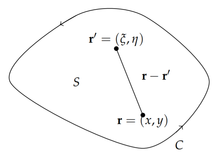
We seek to solve this problem using a Green’s function. As in earlier discussions, the Green’s function satisfies the differential equation and homogeneous boundary conditions. The associated problem is given by

$$\begin{array}{r} \nabla^{2} G=\delta(\xi-x, \eta-y), \quad \text { in } D, \\ G \equiv 0, \quad \text { on } C . \end{array}\label{eq:2}$$

However, we need to be careful as to which variables appear in the differentiation. Many times we just make the adjustment after the derivation of the solution, assuming that the Green’s function is symmetric in its arguments. However, this is not always the case and depends on things such as the self-adjointedness of the problem. Thus, we will assume that the Green’s function satisfies

$$\nabla_{r^{\prime}}^{2} G=\delta(\xi-x, \eta-y),\nonumber$$

where the notation $\nabla_{r^{\prime}}$ means differentiation with respect to the variables $\xi$ and $\eta$. Thus,

$$\nabla_{r^{\prime}}^{2} G=\frac{\partial^{2} G}{\partial \tilde{\xi}^{2}}+\frac{\partial^{2} G}{\partial \eta^{2}}\nonumber$$

With this notation in mind, we now apply Green’s second identity for two dimensions from Problem 8 in Chapter 9. We have

$$\int_{D}\left(u \nabla_{r^{\prime}}^{2} G-G \nabla_{r^{\prime}}^{2} u\right) d A^{\prime}=\int_{C}\left(u \nabla_{r^{\prime}} G-G \nabla_{r^{\prime}} u\right) \cdot d \mathbf{s}^{\prime} .\label{eq:3}$$

Inserting the differential equations, the left hand side of the equation becomes

$$\begin{align} & \int_{D}\left[u \nabla_{r^{\prime}}^{2} G-G \nabla_{r^{\prime}}^{2} u\right] d A^{\prime}\nonumber \\ =& \int_{D}[u(\xi, \eta) \delta(\xi-x, \eta-y)-G(x, y ; \xi, \eta) f(\xi, \eta)] d \xi d \eta\nonumber \\ =& u(x, y)-\int_{D} G(x, y ; \xi, \eta) f(\xi, \eta) d \xi d \eta .\label{eq:4} \end{align}$$

Using the boundary conditions, $u(\xi, \eta)=g(\xi, \eta)$ on $C$ and $G(x, y ; \xi, \eta)=$ 0 on $C$, the right hand side of the equation becomes

$$\int_{C}\left(u \nabla_{r^{\prime}} G-G \nabla_{r^{\prime}} u\right) \cdot d \mathbf{s}^{\prime}=\int_{C} g(\xi, \eta) \nabla_{r^{\prime}} G \cdot d \mathbf{s}^{\prime} .\label{eq:5}$$

Solving for $u(x, y)$, we have the solution written in terms of the Green’s function,

$$u(x, y)=\int_{D} G(x, y ; \xi, \eta) f(\xi, \eta) d \xi d \eta+\int_{C} g(\xi, \eta) \nabla_{r^{\prime}} G \cdot d \mathbf{s}^{\prime} .\nonumber$$

Now we need to find the Green’s function. We find the Green’s functions for several examples.

Example $\PageIndex{1}$

Find the two dimensional Green’s function for the antisymmetric Poisson equation; that is, we seek solutions that are $\theta$-independent.

Solution

The problem we need to solve in order to find the Green’s function involves writing the Laplacian in polar coordinates,

$$v_{r r}+\frac{1}{r} v_{r}=\delta(r) \text {. }\nonumber$$

For $r \neq 0$, this is a Cauchy-Euler type of differential equation. The general solution is $v(r)=A \ln r+B$.

Due to the singularity at $r=0$, we integrate over a domain in which a small circle of radius $\epsilon$ is cut form the plane and apply the two dimensional Divergence Theorem. In particular, we have

$$\begin{align} 1 &=\int_{D_{\epsilon}} \delta(r) d A\nonumber \\ &=\int_{D_{\epsilon}} \nabla^{2} v d A\nonumber \\ &=\int_{C_{\epsilon}} \nabla v \cdots d \mathbf{s}\nonumber \\ &=\int_{C_{\epsilon}} \frac{\partial v}{\partial r} d S=2 \pi A .\label{eq:6} \end{align}$$

Therefore, $A=1 / 2 \pi$. We note that $B$ is arbitrary, so we will take $B=0$ in the remaining discussion.

Using this solution for a source of the form $\delta\left(\mathbf{r}-\mathbf{r}^{\prime}\right)$, we obtain the Green’s function for Poisson’s equation as

$$G\left(\mathbf{r}, \mathbf{r}^{\prime}\right)=\frac{1}{2 \pi} \ln \left|\mathbf{r}-\mathbf{r}^{\prime}\right| .\nonumber$$

Example $\PageIndex{2}$

Find the Green’s function for the infinite plane.

Solution

From Figure $\PageIndex{1}$ we have $\left|\mathbf{r}-\mathbf{r}^{\prime}\right|=\sqrt{(x-\xi)^{2}+(y-\eta)^{2}}$. Therefore, the Green’s function from the last example gives

$$G(x, y, \xi, \eta)=\frac{1}{4 \pi} \ln \left((\xi-x)^{2}+(\eta-y)^{2}\right) .\nonumber$$

Example $\PageIndex{3}$

Find the Green’s function for the half plane, $\{(x, y) \mid y>0\}$, using the Method of Images.

Solution

This problem can be solved using the result for the Green’s function for the infinite plane. We use the Method of Images to construct a function such that $G=0$ on the boundary, $y=0$. Namely, we use the image of the point $(x, y)$ with respect to the $x$-axis, $(x,-y)$.

Imagine that the Green’s function $G(x, y, \xi, \eta)$ represents a point charge at $(x, y)$ and $G(x, y, \xi, \eta)$ provides the electric potential, or response, at $(\xi, \eta)$. This single charge cannot yield a zero potential along the $x$-axis $(y=o)$. One needs an additional charge to yield a zero equipotential line. This is shown in Figure $\PageIndex{2}$.

Figure $\PageIndex{2}$: The Method of Images: The source and image source for the Green’s function for the half plane. Imagine two opposite charges forming a dipole. The electric field lines are depicted indicating that the electric potential, or Green’s function, is constant along $y=0$

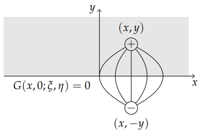
The positive charge has a source of $\delta\left(\mathbf{r}-\mathbf{r}^{\prime}\right)$ at $\mathbf{r}=(x, y)$ and the negative charge is represented by the source $-\delta\left(\mathbf{r}^{*}-\mathbf{r}^{\prime}\right)$ at $\mathbf{r}^{*}=(x,-y)$. We construct the Green’s functions at these two points and introduce a negative sign for the negative image source. Thus, we have

$$G(x, y, \xi, \eta)=\frac{1}{4 \pi} \ln \left((\xi-x)^{2}+(\eta-y)^{2}\right)-\frac{1}{4 \pi} \ln \left((\xi-x)^{2}+(\eta+y)^{2}\right) .\nonumber$$

These functions satisfy the differential equation and the boundary condition

$$G(x, 0, \xi, \eta)=\frac{1}{4 \pi} \ln \left((\xi-x)^{2}+(\eta)^{2}\right)-\frac{1}{4 \pi} \ln \left((\xi-x)^{2}+(\eta)^{2}\right) .\nonumber$$

Example $\PageIndex{4}$

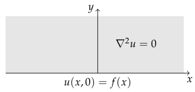
Solve the homogeneous version of the problem; i.e., solve Laplace’s equation on the half plane with a specified value on the boundary.

Solution

We want to solve the problem

$$\begin{align}\nabla^2u=0,&\quad\text{in }D,\nonumber \\ u=f,&\quad\text{on }C,\label{eq:7}\end{align}$$

This is displayed in Figure $\PageIndex{3}$.

Figure $\PageIndex{3}$: This is the domain for a semi-infinite slab with boundary value $u(x, 0)=f(x)$ and governed by Laplace’s equation.

From the previous analysis, the solution takes the form

$$u(x, y)=\int_{C} f \nabla G \cdot \mathbf{n} d s=\int_{C} f \frac{\partial G}{\partial n} d s .\nonumber$$

Since

$$\begin{gathered} G(x, y, \xi, \eta)=\frac{1}{4 \pi} \ln \left((\xi-x)^{2}+(\eta-y)^{2}\right)-\frac{1}{4 \pi} \ln \left((\xi-x)^{2}+(\eta+y)^{2}\right) \\ \frac{\partial G}{\partial n}=\left.\frac{\partial G(x, y, \xi, \eta)}{\partial \eta}\right|_{\eta=0}=\frac{1}{\pi} \frac{y}{(\xi-x)^{2}+y^{2}} \end{gathered}\nonumber$$

We have arrived at the same surface Green’s function as we had found in Example 9.11.2 and the solution is

$$u(x, y)=\frac{1}{\pi} \int_{-\infty}^{\infty} \frac{y}{(x-\xi)^{2}+y^{2}} f(\xi) d \xi .\nonumber$$