9.6: The Convolution Operation

In the list of properties of the Fourier transform, we defined the convolution of two functions, $f(x)$ and $g(x)$ to be the integral

$$(f * g)(x)=\int_{-\infty}^{\infty} f(t) g(x-t) d t .\label{eq:1}$$

In some sense one is looking at a sum of the overlaps of one of the functions and all of the shifted versions of the other function. The German word for convolution is faltung, which means "folding" and in old texts this is referred to as the Faltung Theorem. In this section we will look into the convolution operation and its Fourier transform.

Before we get too involved with the convolution operation, it should be noted that there are really two things you need to take away from this discussion. The rest is detail. First, the convolution of two functions is a new functions as defined by $\eqref{eq:1}$ when dealing wit the Fourier transform. The second and most relevant is that the Fourier transform of the convolution of two functions is the product of the transforms of each function. The rest is all about the use and consequences of these two statements. In this section we will show how the convolution works and how it is useful.

Note

The convolution is commutative.

First, we note that the convolution is commutative: $f * g=g * f$. This is easily shown by replacing $x-t$ with a new variable, $y=x-t$ and $d y=-d t$.

$$\begin{align} (g * f)(x) &=\int_{-\infty}^{\infty} g(t) f(x-t) d t\nonumber \\ &=-\int_{\infty}^{-\infty} g(x-y) f(y) d y\nonumber \\ &=\int_{-\infty}^{\infty} f(y) g(x-y) d y\nonumber \\ &=(f * g)(x) .\label{eq:2} \end{align}$$

The best way to understand the folding of the functions in the convolution is to take two functions and convolve them. The next example gives a graphical rendition followed by a direct computation of the convolution. The reader is encouraged to carry out these analyses for other functions.

Example $\PageIndex{1}$

Graphical Convolution of the box function and a triangle function.

Solution

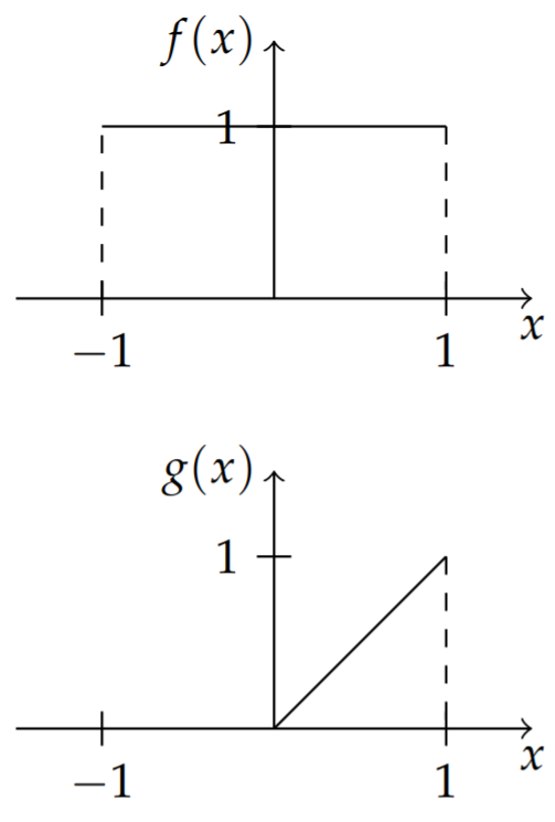
In order to understand the convolution operation, we need to apply it to specific functions. We will first do this graphically for the box function

$$f(x)=\left\{\begin{array}{ll}1,&|x|\leq 1, \\ 0,&|x|>1\end{array}\right.\nonumber$$

and the triangular function

$$g(x)=\left\{\begin{array}{cc}x,&0\leq x\leq 1, \\ 0,&\text{otherwise}\end{array}\right.\nonumber$$

as shown in Figure $\PageIndex{1}$.

Figure $\PageIndex{1}$: A plot of the box function $f(x)$ and the triangle function $g(x)$.

Next, we determine the contributions to the integrand. We consider the shifted and reflected function $g(t-x)$ in Equation $\eqref{eq:1}$ for various values of $t$. For $t=0$, we have $g(x-0)=g(-x)$. This function is a reflection of the triangle function, $g(x)$, as shown in Figure $\PageIndex{2}$.

Figure $\PageIndex{2}$: A plot of the reflected triangle function, $g(-t)$.

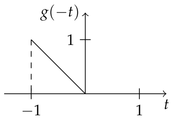
We then translate the triangle function performing horizontal shifts by $t$. In Figure $\PageIndex{3}$ we show such a shifted and reflected $g(x)$ for $t=2$, or $g(2-x)$.

Figure $\PageIndex{3}$: A plot of the reflected triangle function shifted by 2 units, $g(2-t)$.

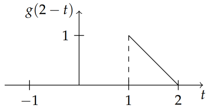
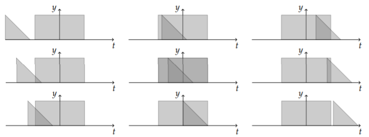
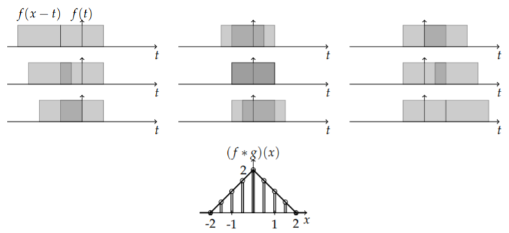
In Figure $\PageIndex{3}$ we show several plots of other shifts, $g(x-t)$, superimposed on $f(x)$.

The integrand is the product of $f(t)$ and $g(x-t)$ and the integral of the product $f(t) g(x-t)$ is given by the sum of the shaded areas for each value of $x$.

In the first plot of Figure $\PageIndex{4}$ the area is zero, as there is no overlap of the functions. Intermediate shift values are displayed in the other plots in Figure $\PageIndex{4}$. The value of the convolution at $x$ is shown by the area under the product of the two functions for each value of $x$.

Figure $\PageIndex{4}$: A plot of the box and triangle functions with the overlap indicated by the shaded area.

Plots of the areas of the convolution of the box and triangle functions for several values of $x$ are given in Figure $\PageIndex{3}$. We see that the value of the convolution integral builds up and then quickly drops to zero as a function of $x$. In Figure $\PageIndex{5}$ the values of these areas is shown as a function of $x$.

Figure $\PageIndex{5}$: Copy and Paste Caption here. (Copyright; author via source)

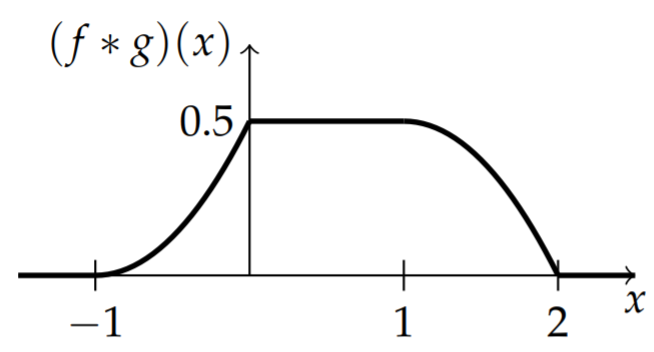
The plot of the convolution in Figure $\PageIndex{5}$ is not easily determined using the graphical method. However, we can directly compute the convolution as shown in the next example.

Example $\PageIndex{2}$

Analytically find the convolution of the box function and the triangle function.

Solution

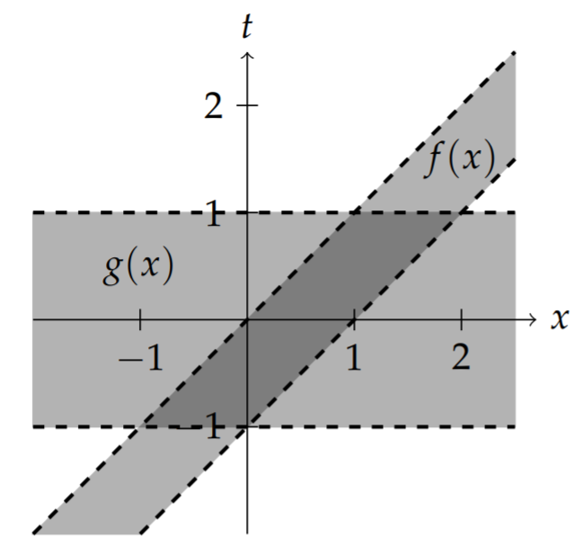
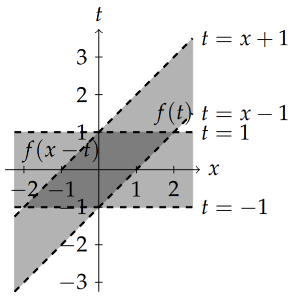
The nonvanishing contributions to the convolution integral are when both $f(t)$ and $g(x-t)$ do not vanish. $f(t)$ is nonzero for $|t| \leq 1$, or $-1 \leq t \leq 1 . g(x-t)$ is nonzero for $0 \leq x-t \leq 1$, or $x-1 \leq t \leq x$. These two regions are shown in Figure $\PageIndex{6}$. On this region, $f(t) g(x-t)=x-t$.

Figure $\PageIndex{6}$: Intersection of the support of $g(x)$ and $f(x)$.

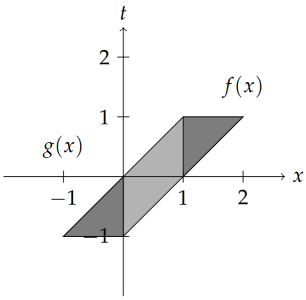
Isolating the intersection in Figure $\PageIndex{7}$, we see in Figure $\PageIndex{7}$ that there are three regions as shown by different shadings. These regions lead to a piecewise defined function with three different branches of nonzero values for $-1<x<0$, $0<x<1$, and $1<x<2$.

Figure $\PageIndex{7}$: Intersection of the support of $g(x)$ and $f(x)$ showing the integration regions.

The values of the convolution can be determined through careful integration. The resulting integrals are given as

$$\begin{align} (f\ast g)(x)&=\int_{-\infty}^\infty f(t)g(x-t)dt\nonumber \\ &=\left\{\begin{array}{ll}\int_{-1}^x (x-t)dt, &-1<x<0 \\ \int_{x-1}^x (x-t)dt, &0<x<1 \\ \int_{x-1}^1(x-t)dt,&1<x<2\end{array}\right.\nonumber \\ &=\left\{\begin{array}{cc}\frac{1}{2}(x+1)^2,&-1<x<0 \\ \frac{1}{2},&0<x<1\\ \frac{1}{2}[1-(x-1)^2]&1<x<2\end{array}\right.\label{eq:3}\end{align}$$

A plot of this function is shown in Figure $\PageIndex{5}$.

Convolution Theorem for Fourier Transforms

In this section we compute the Fourier transform of the convolution integral and show that the Fourier transform of the convolution is the product of the transforms of each function,

$$F[f * g]=\hat{f}(k) \hat{g}(k) .\label{eq:4}$$

First, we use the definitions of the Fourier transform and the convolution to write the transform as

$$\begin{align} F[f * g] &=\int_{-\infty}^{\infty}(f * g)(x) e^{i k x} d x\nonumber \\ &=\int_{-\infty}^{\infty}\left(\int_{-\infty}^{\infty} f(t) g(x-t) d t\right) e^{i k x} d x\nonumber \\ &=\int_{-\infty}^{\infty}\left(\int_{-\infty}^{\infty} g(x-t) e^{i k x} d x\right) f(t) d t .\label{eq:5} \end{align}$$

We now substitute $y=x-t$ on the inside integral and separate the integrals:

$$\begin{align} F[f * g] &=\int_{-\infty}^{\infty}\left(\int_{-\infty}^{\infty} g(x-t) e^{i k x} d x\right) f(t) d t\nonumber \\ &=\int_{-\infty}^{\infty}\left(\int_{-\infty}^{\infty} g(y) e^{i k(y+t)} d y\right) f(t) d t\nonumber \\ &=\int_{-\infty}^{\infty}\left(\int_{-\infty}^{\infty} g(y) e^{i k y} d y\right) f(t) e^{i k t} d t\nonumber \\ &=\left(\int_{-\infty}^{\infty} f(t) e^{i k t} d t\right)\left(\int_{-\infty}^{\infty} g(y) e^{i k y} d y\right)\label{eq:6} \end{align}$$

We see that the two integrals are just the Fourier transforms of $f$ and $g$. Therefore, the Fourier transform of a convolution is the product of the Fourier transforms of the functions involved:

$$F[f * g]=\hat{f}(k) \hat{g}(k) \text {. }\nonumber$$

Example $\PageIndex{3}$

Compute the convolution of the box function of height one and width two with itself.

Solution

Let $\hat{f}(k)$ be the Fourier transform of $f(x)$. Then, the Convolution Theorem says that $F[f * f](k)=\hat{f}^{2}(k)$, or

$$(f * f)(x)=F^{-1}\left[\hat{f}^{2}(k)\right] .\nonumber$$

For the box function, we have already found that

$$\hat{f}(k)=\frac{2}{k} \sin k .\nonumber$$

So, we need to compute

$$\begin{align} (f * f)(x) &=F^{-1}\left[\frac{4}{k^{2}} \sin ^{2} k\right]\nonumber \\ &=\frac{1}{2 \pi} \int_{-\infty}^{\infty}\left(\frac{4}{k^{2}} \sin ^{2} k\right) e^{-i k x} d k .\label{eq:7} \end{align}$$

One way to compute this integral is to extend the computation into the complex $k$-plane. We first need to rewrite the integrand. Thus,

$$\begin{align} (f * f)(x) &=\frac{1}{2 \pi} \int_{-\infty}^{\infty} \frac{4}{k^{2}} \sin ^{2} k e^{-i k x} d k\nonumber \\ &=\frac{1}{\pi} \int_{-\infty}^{\infty} \frac{1}{k^{2}}[1-\cos 2 k] e^{-i k x} d k\nonumber \\ &=\frac{1}{\pi} \int_{-\infty}^{\infty} \frac{1}{k^{2}}\left[1-\frac{1}{2}\left(e^{i k}+e^{-i k}\right)\right] e^{-i k x} d k\nonumber \\ &=\frac{1}{\pi} \int_{-\infty}^{\infty} \frac{1}{k^{2}}\left[e^{-i k x}-\frac{1}{2}\left(e^{-i(1-k)}+e^{-i(1+k)}\right)\right] d k .\label{eq:8} \end{align}$$

We can compute the above integrals if we know how to compute the integral

$$I(y)=\frac{1}{\pi} \int_{-\infty}^{\infty} \frac{e^{-i k y}}{k^{2}} d k .\nonumber$$

Then, the result can be found in terms of $I(y)$ as

$$(f * f)(x)=I(x)-\frac{1}{2}[I(1-k)+I(1+k)] .\nonumber$$

We consider the integral

$$\oint_{C} \frac{e^{-i y z}}{\pi z^{2}} d z\nonumber$$

over the contour in Figure $\PageIndex{8}$.

Figure $\PageIndex{8}$: Contour for computing $P \int_{-\infty}^{\infty} \frac{e^{-i y z}}{\pi z^{2}} d z$.

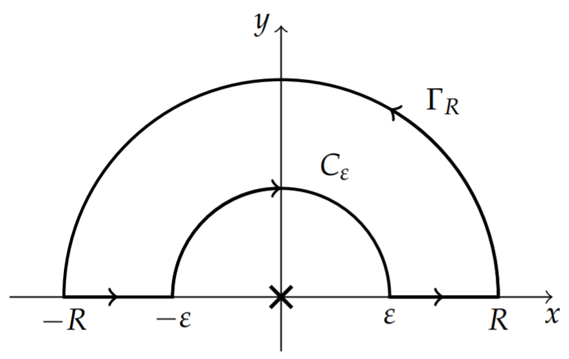
We can see that there is a double pole at $z = 0$. The pole is on the real axis. So, we will need to cut out the pole as we seek the value of the principal value integral.

Recall from Chapter 8 that

$$\oint_{C_R}\frac{e^{-iyz}}{\pi z^2}dz=\int_{\Gamma_R}\frac{e^{-iyz}}{\pi z^2}dz+\int_{-R}^{-\epsilon}\frac{e^{-iyz}}{\pi z^2}dz+\int_{C_e}\frac{e^{-iyz}}{\pi z^2}dz+\int_\epsilon^R\frac{e^{-iyz}}{\pi z^2}dz.\nonumber$$

The integral $\oint_{C_{R}} \frac{e^{-i y z}}{\pi z^{2}} d z$ vanishes since there are no poles enclosed in the contour! The sum of the second and fourth integrals gives the integral we seek as $\epsilon \rightarrow 0$ and $R \rightarrow \infty$. The integral over $\Gamma_{R}$ will vanish as $R$ gets large according to Jordan’s Lemma provided $y<0$. That leaves the integral over the small semicircle.

As before, we can show that

$$\lim _{\epsilon \rightarrow 0} \int_{\mathcal{C}_{\epsilon}} f(z) d z=-\pi i \operatorname{Res}[f(z) ; z=0] .\nonumber$$

Therefore, we find

$$I(y)=P \int_{-\infty}^{\infty} \frac{e^{-i y z}}{\pi z^{2}} d z=\pi i \operatorname{Res}\left[\frac{e^{-i y z}}{\pi z^{2}} ; z=0\right] .\nonumber$$

A simple computation of the reside gives $I(y)=-y$, for $y<0$.

When $y>0$, we need to close the contour in the lower half plane in order to apply Jordan’s Lemma. Carrying out the computation, one finds $I(y)=y$, for $y>0$. Thus,

$$I(y)=\left\{\begin{array}{cc} -y, & y>0, \\ y, & y<0, \end{array}\right.\label{eq:9}$$

We are now ready to finish the computation of the convolution. We have to combine the integrals $I(y), I(y+1)$, and $I(y-1)$, since $(f * f)(x)=I(x)-$ $\frac{1}{2}[I(1-k)+I(1+k)]$. This gives different results in four intervals:

$$\begin{align} (f * f)(x) &=x-\frac{1}{2}[(x-2)+(x+2)]=0, \quad x<-2,\nonumber \\ &=x-\frac{1}{2}[(x-2)-(x+2)]=2+x \quad-2<x<0,\nonumber \\ &=-x-\frac{1}{2}[(x-2)-(x+2)]=2-x, \quad 0<x<2,\nonumber \\ &=-x-\frac{1}{2}[-(x-2)-(x+2)]=0, \quad x>2 .\label{eq:10} \end{align}$$

A plot of this solution is the triangle function,

$$(f * f)(x)=\left\{\begin{array}{cc} 0, & x<-2 \\ 2+x, & -2<x<0 \\ 2-x, & 0<x<2 \\ 0, & x>2 \end{array}\right.\label{eq:11}$$

which was shown in the last example.

Example $\PageIndex{4}$

Find the convolution of the box function of height one and width two with itself using a direct computation of the convolution integral.

Solution

The nonvanishing contributions to the convolution integral are when both $f(t)$ and $f(x-t)$ do not vanish. $f(t)$ is nonzero for $|t| \leq 1$, or $-1 \leq t \leq 1 . f(x-t)$ is nonzero for $|x-t| \leq 1$, or $x-1 \leq t \leq x+1$. These two regions are shown in Figure $\PageIndex{10}$. On this region, $f(t) g(x-t)=1$.

Figure $\PageIndex{9}$: Plot of the regions of support for $f(t)$ and $f(x-t)$.

Figure $\PageIndex{10}$: A plot of the convolution of a box function with itself. The areas of the overlaps of as $f(x-t)$ is translated across $f(t)$ are shown as well. The result is the triangular function.

Thus, the nonzero contributions to the convolution are

$$(f * f)(x)=\left\{\begin{array}{l} \int_{-1}^{x+1} d t, \quad 0 \leq x \leq 2, \\ \int_{x-1}^{1} d t, \quad-2 \leq x \leq 0, \end{array}=\left\{\begin{array}{cc} 2+x, & 0 \leq x \leq 2, \\ 2-x, & -2 \leq x \leq 0 . \end{array}\right.\right.\nonumber$$

Once again, we arrive at the triangle function.

In the last section we showed the graphical convolution. For completeness, we do the same for this example. In Figure $\PageIndex{10}$ we show the results. We see that the convolution of two box functions is a triangle function.

Example $\PageIndex{5}$

Show the graphical convolution of the box function of height one and width two with itself.

Let’s consider a slightly more complicated example, the convolution of two Gaussian functions.

Example $\PageIndex{6}$

Convolution of two Gaussian functions $f(x)=e^{-ax^2}$.

Solution

In this example we will compute the convolution of two Gaussian functions with different widths. Let $f(x)=e^{-a x^{2}}$ and $g(x)=e^{-b x^{2}}$. A direct evaluation of the integral would be to compute

$$(f * g)(x)=\int_{-\infty}^{\infty} f(t) g(x-t) d t=\int_{-\infty}^{\infty} e^{-a t^{2}-b(x-t)^{2}} d t .\nonumber$$

This integral can be rewritten as

$$(f * g)(x)=e^{-b x^{2}} \int_{-\infty}^{\infty} e^{-(a+b) t^{2}+2 b x t} d t .\nonumber$$

One could proceed to complete the square and finish carrying out the integration. However, we will use the Convolution Theorem to evaluate the convolution and leave the evaluation of this integral to Problem 12.

Recalling the Fourier transform of a Gaussian from Example 9.5.1, we have

$$\hat{f}(k)=F[e^{-ax^2}]=\sqrt{\frac{\pi}{a}}e^{-k^2/4a}\label{eq:12}$$

and

$$\hat{g}(k)=F[e^{-bx^2}]=\sqrt{\frac{\pi}{b}}e^{-k^2/4b}.\nonumber$$

Denoting the convolution function by $h(x) = (f ∗ g)(x)$, the Convolution Theorem gives

$$\hat{h}(k)=\hat{f}(k)\hat{g}(k)=\frac{\pi}{\sqrt{ab}}e^{-k^2/4a}e^{-k^2/4b}.\nonumber$$

This is another Gaussian function, as seen by rewriting the Fourier transform of $h(x)$ as

$$\hat{h}(k)=\frac{\pi}{\sqrt{ab}}e^{-\frac{1}{4}\left(\frac{1}{a}+\frac{1}{b}\right)k^2}=\frac{\pi}{\sqrt{ab}}e^{-\frac{a+b}{4ab}k^2}.\label{eq:13}$$

In order to complete the evaluation of the convolution of these two Gaussian functions, we need to find the inverse transform of the Gaussian in Equation $\eqref{eq:13}$. We can do this by looking at Equation $\eqref{eq:12}$. We have first that

$$F^{-1}\left[\sqrt{\frac{\pi}{a}}e^{-k^2/4a}\right]=e^{-ax^2}.\nonumber$$

Moving the constants, we then obtain

$$F^{-1}[e^{-k^2/4a}]=\sqrt{\frac{a}{\pi}}e^{-ax^2}.\nonumber$$

We now make the substitution $\alpha =\frac{1}{4a}$,

$$F^{-1}[e^{-\alpha k^2}]=\sqrt{\frac{1}{4\pi\alpha}}e^{-x^2/4\alpha}.\nonumber$$

This is in the form needed to invert $\eqref{eq:13}$. Thus, for $\alpha =\frac{a+b}{4ab}$ we find

$$(f * g)(x)=h(x)=\sqrt{\frac{\pi}{a+b}} e^{-\frac{a b}{a+b} x^{2}} .\nonumber$$

Application to Signal Analysis

There are many applications of the convolution operation. One of these areas is the study of analog signals. An analog signal is a continuous signal and may contain either a finite, or continuous, set of frequencies. Fourier transforms can be used to represent such signals as a sum over the frequency content of these signals. In this section we will describe how convolutions can be used in studying signal analysis.

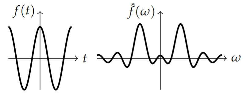
The first application is filtering. For a given signal there might be some noise in the signal, or some undesirable high frequencies. For example, a device used for recording an analog signal might naturally not be able to record high frequencies. Let $f(t)$ denote the amplitude of a given analog signal and $\hat{f}(\omega)$ be the Fourier transform of this signal such the example provided in Figure $\PageIndex{11}$. Recall that the Fourier transform gives the frequency content of the signal.

Figure $\PageIndex{11}$: Schematic plot of a signal $f(t)$ and its Fourier transform $\hat{f}(\omega )$.

There are many ways to filter out unwanted frequencies. The simplest would be to just drop all of the high (angular) frequencies. For example, for some cutoff frequency $\omega_{0}$ frequencies $|\omega|>\omega_{0}$ will be removed. The Fourier transform of the filtered signal would then be zero for $|\omega|>\omega_{0}$. This could be accomplished by multiplying the Fourier transform of the signal by a function that vanishes for $|\omega|>\omega_{0}$. For example, we could use the gate function

$$p_{\omega_{0}}(\omega)=\left\{\begin{array}{ll} 1, & |\omega| \leq \omega_{0} \\ 0, & |\omega|>\omega_{0} \end{array},\right.\label{eq:14}$$

as shown in Figure $\PageIndex{12}$.

Figure $\PageIndex{12}$: (a) Plot of the Fourier transform $f(\omega)$ of a signal. (b) The gate function $p_{\omega_{0}}(\omega)$ used to filter out high frequencies. (c) The product of the functions, $\hat{g}(\omega)=\hat{f}(\omega) p_{\omega_{0}}(\omega)$, in (a) and (b) shows how the filters cuts out high frequencies, $|\omega|>\omega_{0}$.

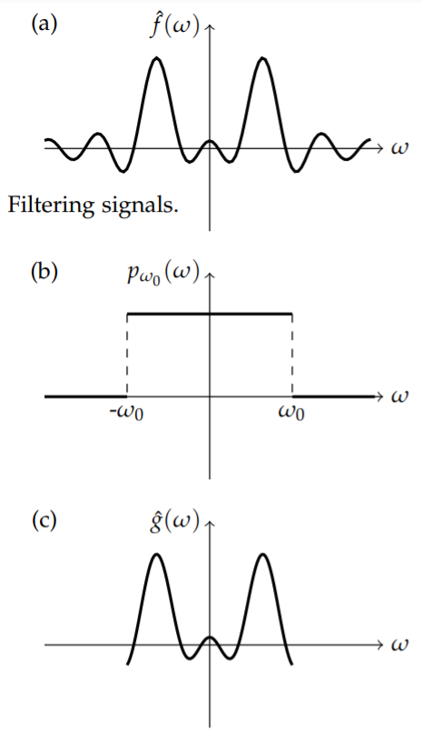
In general, we multiply the Fourier transform of the signal by some filtering function $\hat{h}(t)$ to get the Fourier transform of the filtered signal,

$$\hat{g}(\omega)=\hat{f}(\omega) \hat{h}(\omega) .\nonumber$$

The new signal, $g(t)$ is then the inverse Fourier transform of this product, giving the new signal as a convolution:

$$g(t)=F^{-1}[\hat{f}(\omega) \hat{h}(\omega)]=\int_{-\infty}^{\infty} h(t-\tau) f(\tau) d \tau .\label{eq:15}$$

Such processes occur often in systems theory as well. One thinks of $f(t)$ as the input signal into some filtering device which in turn produces the output, $g(t)$. The function $h(t)$ is called the impulse response. This is because it is a response to the impulse function, $\delta(t)$. In this case, one has

$$\int_{-\infty}^{\infty} h(t-\tau) \delta(\tau) d \tau=h(t) .\nonumber$$

Another application of the convolution is in windowing. This represents what happens when one measures a real signal. Real signals cannot be recorded for all values of time. Instead data is collected over a finite time interval. If the length of time the data is collected is $T$, then the resulting signal is zero outside this time interval. This can be modeled in the same way as with filtering, except the new signal will be the product of the old signal with the windowing function. The resulting Fourier transform of the new signal will be a convolution of the Fourier transforms of the original signal and the windowing function.

Example $\PageIndex{7}$: Finite Wave Train, Revisited

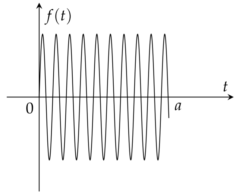
We return to the finite wave train in Example 9.5.6 given by

$$h(t)=\left\{\begin{array}{cl} \cos \omega_{0} t, & |t| \leq a \\ 0, & |t|>a \end{array} .\right.\nonumber$$

Solution

We can view this as a windowed version of $f(t)=\cos \omega_{0}$ t obtained by multiplying $f(t)$ by the gate function

$$g_a(t)=\left\{\begin{array}{rl}1,&|x|\leq a \\ 0,&|x|>a\end{array}\right.\label{eq:16}$$

This is shown in Figure $\PageIndex{13}$. Then, the Fourier transform is given as a convolution,

$$\begin{align} \hat{h}(\omega) &=\left(\hat{f} * \hat{g}_{a}\right)(\omega)\nonumber \\ &=\frac{1}{2 \pi} \int_{-\infty}^{\infty} \hat{f}(\omega-v) \hat{g}_{a}(v) d v .\label{eq:17} \end{align}$$

Note that the convolution in frequency space requires the extra factor of $1 /(2 \pi)$.

Figure $\PageIndex{13}$: A plot of the finite wave train.

Note

The convolution in spectral space is defined with an extra factor of $1 / 2 \pi$ so as to preserve the idea that the inverse Fourier transform of a convolution is the product of the corresponding signals.

We need the Fourier transforms of $f$ and $g_{a}$ in order to finish the computation. The Fourier transform of the box function was found in Example 9.5.2 as

$$\hat{g}_{a}(\omega)=\frac{2}{\omega} \sin \omega a \text {. }\nonumber$$

The Fourier transform of the cosine function, $f(t)=\cos \omega_{0} t$, is

$$\begin{align} \hat{f}(\omega) &=\int_{-\infty}^{\infty} \cos \left(\omega_{0} t\right) e^{i \omega t} d t\nonumber \\ &=\int_{-\infty}^{\infty} \frac{1}{2}\left(e^{i \omega_{0} t}+e^{-i \omega_{0} t}\right) e^{i \omega t} d t\nonumber \\ &=\frac{1}{2} \int_{-\infty}^{\infty}\left(e^{i\left(\omega+\omega_{0}\right) t}+e^{i\left(\omega-\omega_{0}\right) t}\right) d t\nonumber \\ &=\pi\left[\delta\left(\omega+\omega_{0}\right)+\delta\left(\omega-\omega_{0}\right)\right]\label{eq:18} \end{align}$$

Note that we had earlier computed the inverse Fourier transform of this function in Example 9.5.5.

Inserting these results in the convolution integral, we have

$$\begin{align} \hat{h}(\omega) &=\frac{1}{2 \pi} \int_{-\infty}^{\infty} \hat{f}(\omega-v) \hat{g}_{a}(v) d v\nonumber \\ &=\frac{1}{2 \pi} \int_{-\infty}^{\infty} \pi\left[\delta\left(\omega-v+\omega_{0}\right)+\delta\left(\omega-v-\omega_{0}\right)\right] \frac{2}{v} \sin v a d v\nonumber \\ &=\frac{\sin \left(\omega+\omega_{0}\right) a}{\omega+\omega_{0}}+\frac{\sin \left(\omega-\omega_{0}\right) a}{\omega-\omega_{0}} .\label{eq:19} \end{align}$$

This is the same result we had obtained in Example 9.5.6.

Parseval’s Equality

Note

The integral/sum of the (modulus) square of a function is the integral/sum of the (modulus) square of the transform.

As another example of the convolution theorem, we derive Parseval’s Equality (named after Marc-Antoine Parseval (1755-1836)):

$$\int_{-\infty}^{\infty}|f(t)|^{2} d t=\frac{1}{2 \pi} \int_{-\infty}^{\infty}|\hat{f}(\omega)|^{2} d \omega .\label{eq:20}$$

This equality has a physical meaning for signals. The integral on the left side is a measure of the energy content of the signal in the time domain. The right side provides a measure of the energy content of the transform of the signal. Parseval’s equality, is simply a statement that the energy is invariant under the Fourier transform. Parseval’s equality is a special case of Plancherel’s formula (named after Michel Plancherel, 1885-1967).

Let’s rewrite the Convolution Theorem in its inverse form

$$F^{-1}[\hat{f}(k) \hat{g}(k)]=(f * g)(t) .\label{eq:21}$$

Then, by the definition of the inverse Fourier transform, we have

$$\int_{-\infty}^{\infty} f(t-u) g(u) d u=\frac{1}{2 \pi} \int_{-\infty}^{\infty} \hat{f}(\omega) \hat{g}(\omega) e^{-i \omega t} d \omega .\nonumber$$

Setting $t=0$,

$$\int_{-\infty}^{\infty} f(-u) g(u) d u=\frac{1}{2 \pi} \int_{-\infty}^{\infty} \hat{f}(\omega) \hat{g}(\omega) d \omega .\label{eq:22}$$

Now, let $g(t)=\overline{f(-t)}$, or $f(-t)=\overline{g(t)}$. We note that the Fourier transform of $g(t)$ is related to the Fourier transform of $f(t)$ :

$$\begin{align} \hat{g}(\omega) &=\int_{-\infty}^{\infty} \overline{f(-t)} e^{i \omega t} d t\nonumber \\ &=-\int_{\infty}^{-\infty} \overline{f(\tau) e^{-i \omega \tau}} d \tau\nonumber \\ &=\int_{-\infty}^{\infty} f(\tau) e^{i \omega \tau} d \tau=\bar{f}(\omega) .\label{eq:23} \end{align}$$

So, inserting this result into Equation $\eqref{eq:22}$, we find that

$$\int_{-\infty}^{\infty} f(-u) \overline{f(-u)} d u=\frac{1}{2 \pi} \int_{-\infty}^{\infty}|\hat{f}(\omega)|^{2} d \omega\nonumber$$

which yields Parseval’s Equality in the form $\eqref{eq:20}$ after substituting $t=-u$ on the left.

As noted above, the forms in Equations $\eqref{eq:20}$ and $\eqref{eq:22}$ are often referred to as the Plancherel formula or Parseval formula. A more commonly defined Parseval equation is that given for Fourier series. For example, for a function $f(x)$ defined on $[-\pi, \pi]$, which has a Fourier series representation, we have

$$\frac{a_{0}^{2}}{2}+\sum_{n=1}^{\infty}\left(a_{n}^{2}+b_{n}^{2}\right)=\frac{1}{\pi} \int_{-\pi}^{\pi}[f(x)]^{2} d x .\nonumber$$

In general, there is a Parseval identity for functions that can be expanded in a complete sets of orthonormal functions, $\left\{\phi_{n}(x)\right\}, n=1,2, \ldots$, which is given by

$$\sum_{n=1}^{\infty}<f, \phi_{n}>^{2}=\|f\|^{2} .\nonumber$$

Here $\|f\|^{2}=\langle f, f\rangle$. The Fourier series example is just a special case of this formula.