9.8: Applications of Laplace Transforms
- Page ID
- 90977

\( \newcommand{\vecs}[1]{\overset { \scriptstyle \rightharpoonup} {\mathbf{#1}} } \)
\( \newcommand{\vecd}[1]{\overset{-\!-\!\rightharpoonup}{\vphantom{a}\smash {#1}}} \)
\( \newcommand{\id}{\mathrm{id}}\) \( \newcommand{\Span}{\mathrm{span}}\)
( \newcommand{\kernel}{\mathrm{null}\,}\) \( \newcommand{\range}{\mathrm{range}\,}\)
\( \newcommand{\RealPart}{\mathrm{Re}}\) \( \newcommand{\ImaginaryPart}{\mathrm{Im}}\)
\( \newcommand{\Argument}{\mathrm{Arg}}\) \( \newcommand{\norm}[1]{\| #1 \|}\)
\( \newcommand{\inner}[2]{\langle #1, #2 \rangle}\)
\( \newcommand{\Span}{\mathrm{span}}\)
\( \newcommand{\id}{\mathrm{id}}\)
\( \newcommand{\Span}{\mathrm{span}}\)
\( \newcommand{\kernel}{\mathrm{null}\,}\)
\( \newcommand{\range}{\mathrm{range}\,}\)
\( \newcommand{\RealPart}{\mathrm{Re}}\)
\( \newcommand{\ImaginaryPart}{\mathrm{Im}}\)
\( \newcommand{\Argument}{\mathrm{Arg}}\)
\( \newcommand{\norm}[1]{\| #1 \|}\)
\( \newcommand{\inner}[2]{\langle #1, #2 \rangle}\)
\( \newcommand{\Span}{\mathrm{span}}\) \( \newcommand{\AA}{\unicode[.8,0]{x212B}}\)
\( \newcommand{\vectorA}[1]{\vec{#1}} % arrow\)
\( \newcommand{\vectorAt}[1]{\vec{\text{#1}}} % arrow\)
\( \newcommand{\vectorB}[1]{\overset { \scriptstyle \rightharpoonup} {\mathbf{#1}} } \)
\( \newcommand{\vectorC}[1]{\textbf{#1}} \)
\( \newcommand{\vectorD}[1]{\overrightarrow{#1}} \)
\( \newcommand{\vectorDt}[1]{\overrightarrow{\text{#1}}} \)
\( \newcommand{\vectE}[1]{\overset{-\!-\!\rightharpoonup}{\vphantom{a}\smash{\mathbf {#1}}}} \)
\( \newcommand{\vecs}[1]{\overset { \scriptstyle \rightharpoonup} {\mathbf{#1}} } \)
\( \newcommand{\vecd}[1]{\overset{-\!-\!\rightharpoonup}{\vphantom{a}\smash {#1}}} \)
\(\newcommand{\avec}{\mathbf a}\) \(\newcommand{\bvec}{\mathbf b}\) \(\newcommand{\cvec}{\mathbf c}\) \(\newcommand{\dvec}{\mathbf d}\) \(\newcommand{\dtil}{\widetilde{\mathbf d}}\) \(\newcommand{\evec}{\mathbf e}\) \(\newcommand{\fvec}{\mathbf f}\) \(\newcommand{\nvec}{\mathbf n}\) \(\newcommand{\pvec}{\mathbf p}\) \(\newcommand{\qvec}{\mathbf q}\) \(\newcommand{\svec}{\mathbf s}\) \(\newcommand{\tvec}{\mathbf t}\) \(\newcommand{\uvec}{\mathbf u}\) \(\newcommand{\vvec}{\mathbf v}\) \(\newcommand{\wvec}{\mathbf w}\) \(\newcommand{\xvec}{\mathbf x}\) \(\newcommand{\yvec}{\mathbf y}\) \(\newcommand{\zvec}{\mathbf z}\) \(\newcommand{\rvec}{\mathbf r}\) \(\newcommand{\mvec}{\mathbf m}\) \(\newcommand{\zerovec}{\mathbf 0}\) \(\newcommand{\onevec}{\mathbf 1}\) \(\newcommand{\real}{\mathbb R}\) \(\newcommand{\twovec}[2]{\left[\begin{array}{r}#1 \\ #2 \end{array}\right]}\) \(\newcommand{\ctwovec}[2]{\left[\begin{array}{c}#1 \\ #2 \end{array}\right]}\) \(\newcommand{\threevec}[3]{\left[\begin{array}{r}#1 \\ #2 \\ #3 \end{array}\right]}\) \(\newcommand{\cthreevec}[3]{\left[\begin{array}{c}#1 \\ #2 \\ #3 \end{array}\right]}\) \(\newcommand{\fourvec}[4]{\left[\begin{array}{r}#1 \\ #2 \\ #3 \\ #4 \end{array}\right]}\) \(\newcommand{\cfourvec}[4]{\left[\begin{array}{c}#1 \\ #2 \\ #3 \\ #4 \end{array}\right]}\) \(\newcommand{\fivevec}[5]{\left[\begin{array}{r}#1 \\ #2 \\ #3 \\ #4 \\ #5 \\ \end{array}\right]}\) \(\newcommand{\cfivevec}[5]{\left[\begin{array}{c}#1 \\ #2 \\ #3 \\ #4 \\ #5 \\ \end{array}\right]}\) \(\newcommand{\mattwo}[4]{\left[\begin{array}{rr}#1 \amp #2 \\ #3 \amp #4 \\ \end{array}\right]}\) \(\newcommand{\laspan}[1]{\text{Span}\{#1\}}\) \(\newcommand{\bcal}{\cal B}\) \(\newcommand{\ccal}{\cal C}\) \(\newcommand{\scal}{\cal S}\) \(\newcommand{\wcal}{\cal W}\) \(\newcommand{\ecal}{\cal E}\) \(\newcommand{\coords}[2]{\left\{#1\right\}_{#2}}\) \(\newcommand{\gray}[1]{\color{gray}{#1}}\) \(\newcommand{\lgray}[1]{\color{lightgray}{#1}}\) \(\newcommand{\rank}{\operatorname{rank}}\) \(\newcommand{\row}{\text{Row}}\) \(\newcommand{\col}{\text{Col}}\) \(\renewcommand{\row}{\text{Row}}\) \(\newcommand{\nul}{\text{Nul}}\) \(\newcommand{\var}{\text{Var}}\) \(\newcommand{\corr}{\text{corr}}\) \(\newcommand{\len}[1]{\left|#1\right|}\) \(\newcommand{\bbar}{\overline{\bvec}}\) \(\newcommand{\bhat}{\widehat{\bvec}}\) \(\newcommand{\bperp}{\bvec^\perp}\) \(\newcommand{\xhat}{\widehat{\xvec}}\) \(\newcommand{\vhat}{\widehat{\vvec}}\) \(\newcommand{\uhat}{\widehat{\uvec}}\) \(\newcommand{\what}{\widehat{\wvec}}\) \(\newcommand{\Sighat}{\widehat{\Sigma}}\) \(\newcommand{\lt}{<}\) \(\newcommand{\gt}{>}\) \(\newcommand{\amp}{&}\) \(\definecolor{fillinmathshade}{gray}{0.9}\)Although the Laplace transform is a very useful transform, it is often encountered only as a method for solving initial value problems in introductory differential equations. In this section we will show how to solve simple differential equations. Along the way we will introduce step and impulse functions and show how the Convolution Theorem for Laplace transforms plays a role in finding solutions. However, we will first explore an unrelated application of Laplace transforms. We will see that the Laplace transform is useful in finding sums of infinite series.
Series Summation Using Laplace Transforms
We saw in Chapter ?? that Fourier series can be used to sum series. For example, in Problem ??.13, one proves that
\[\sum_{n=1}^{\infty} \frac{1}{n^{2}}=\frac{\pi^{2}}{6} .\nonumber \]
In this section we will show how Laplace transforms can be used to sum series.\(^{1}\) There is an interesting history of using integral transforms to sum series. For example, Richard Feynman\(^{2}\) \((1918-1988)\) described how one can use the convolution theorem for Laplace transforms to sum series with denominators that involved products. We will describe this and simpler sums in this section.
We begin by considering the Laplace transform of a known function,
\[F(s)=\int_{0}^{\infty} f(t) e^{-s t} d t .\nonumber \]
Inserting this expression into the sum \(\sum_{n} F(n)\) and interchanging the sum and integral, we find
\[\begin{align} \sum_{n=0}^{\infty} F(n) &=\sum_{n=0}^{\infty} \int_{0}^{\infty} f(t) e^{-n t} d t\nonumber \\ &=\int_{0}^{\infty} f(t) \sum_{n=0}^{\infty}\left(e^{-t}\right)^{n} d t\nonumber \\ &=\int_{0}^{\infty} f(t) \frac{1}{1-e^{-t}} d t .\label{eq:1} \end{align} \]
The last step was obtained using the sum of a geometric series. The key is being able to carry out the final integral as we show in the next example.
Evaluate the sum \(\sum_{n=1}^{\infty} \frac{(-1)^{n+1}}{n}\).
Solution
Since, \(\mathcal{L}[1]=1 / \mathrm{s}\), we have
\[\begin{align} \sum_{n=1}^{\infty} \frac{(-1)^{n+1}}{n} &=\sum_{n=1}^{\infty} \int_{0}^{\infty}(-1)^{n+1} e^{-n t} d t\nonumber \\ &=\int_{0}^{\infty} \frac{e^{-t}}{1+e^{-t}} d t\nonumber \\ &=\int_{1}^{2} \frac{d u}{u}=\ln 2\label{eq:2} \end{align} \]
Evaluate the sum \(\sum_{n=1}^{\infty} \frac{1}{n^{2}}\).
Solution
This is a special case of the Riemann zeta function
\[\zeta(s)=\sum_{n=1}^{\infty} \frac{1}{n^{s}} .\label{eq:3} \]
The Riemann zeta function\(^{3}\) is important in the study of prime numbers and more recently has seen applications in the study of dynamical systems. The series in this example is \(\zeta(2)\). We have already seen in ??.13 that
\[\zeta(2)=\frac{\pi^{2}}{6} .\nonumber \]
Using Laplace transforms, we can provide an integral representation of \(\zeta(2)\).
The first step is to find the correct Laplace transform pair. The sum involves the function \(F(n)=1 / n^{2}\). So, we look for a function \(f(t)\) whose Laplace transform is \(F(s)=1 / s^{2}\). We know by now that the inverse Laplace transform of \(F(s)=1 / s^{2}\) is \(f(t)=t\). As before, we replace each term in the series by a Laplace transform, exchange the summation and integration, and sum the resulting geometric series:
\[\begin{align} \sum_{n=1}^{\infty} \frac{1}{n^{2}} &=\sum_{n=1}^{\infty} \int_{0}^{\infty} t e^{-n t} d t\nonumber \\ &=\int_{0}^{\infty} \frac{t}{e^{t}-1} d t .\label{eq:4} \end{align} \]
So, we have that
\[\int_{0}^{\infty} \frac{t}{e^{t}-1} d t=\sum_{n=1}^{\infty} \frac{1}{n^{2}}=\zeta(2)\nonumber \]
Integrals of this type occur often in statistical mechanics in the form of Bose-Einstein integrals. These are of the form
\[G_{n}(z)=\int_{0}^{\infty} \frac{x^{n-1}}{z^{-1} e^{x}-1} d x .\nonumber \]
Note that \(G_{n}(1)=\Gamma(n) \zeta(n)\).
A translation of Riemann, Bernhard (1859), "Über die Anzahl der Primzahlen unter einer gegebenen Grösse" is in H. M. Edwards (1974). Riemann’s Zeta Function. Academic Press. Riemann had shown that the Riemann zeta function can be obtained through contour integral representation, \(2 \sin (\pi s) \Gamma \zeta(s)=\) \(i \oint_{C} \frac{(-x)^{s-1}}{e^{x}-1} d x\), for a specific contour \(C\).
In general the Riemann zeta function has to be tabulated through other means. In some special cases, one can closed form expressions. For example,
\[\zeta(2 n)=\frac{2^{2 n-1} \pi^{2 n}}{(2 n) !} B_{n},\nonumber \]
where the \(B_{n}\) ’s are the Bernoulli numbers. Bernoulli numbers are defined through the Maclaurin series expansion
\[\frac{x}{e^{x}-1}=\sum_{n=0}^{\infty} \frac{B_{n}}{n !} x^{n} .\nonumber \]
The first few Riemann zeta functions are
\[\zeta(2)=\frac{\pi^{2}}{6}, \quad \zeta(4)=\frac{\pi^{4}}{90}, \quad \zeta(6)=\frac{\pi^{6}}{945} .\nonumber \]
We can extend this method of using Laplace transforms to summing series whose terms take special general forms. For example, from Feynman’s 1949 paper we note that
\[\frac{1}{(a+b n)^{2}}=-\frac{\partial}{\partial a} \int_{0}^{\infty} e^{-s(a+b n)} d s .\nonumber \]
This identity can be shown easily by first noting
\[\int_{0}^{\infty} e^{-s(a+b n)} d s=\left[\frac{-e^{-s(a+b n)}}{a+b n}\right]_{0}^{\infty}=\frac{1}{a+b n} .\nonumber \]
Now, differentiate the result with respect to \(a\) and the result follows.
The latter identity can be generalized further as
\[\frac{1}{(a+b n)^{k+1}}=\frac{(-1)^{k}}{k !} \frac{\partial^{k}}{\partial a^{k}} \int_{0}^{\infty} e^{-s(a+b n)} d s .\nonumber \]
In Feynman’s 1949 paper, he develops methods for handling several other general sums using the convolution theorem. Wheelon gives more examples of these. We will just provide one such result and an example. First, we note that
\[\frac{1}{a b}=\int_{0}^{1} \frac{d u}{[a(1-u)+b u]^{2}} .\nonumber \]
However,
\[\frac{1}{[a(1-u)+b u]^{2}}=\int_{0}^{\infty} t e^{-t[a(1-u)+b u]} d t .\nonumber \]
So, we have
\[\frac{1}{a b}=\int_{0}^{1} d u \int_{0}^{\infty} t e^{-t[a(1-u)+b u]} d t .\nonumber \]
We see in the next example how this representation can be useful.
Evaluate \(\sum_{n=0}^{\infty} \frac{1}{(2 n+1)(2 n+2)}\).
Solution
We sum this series by first letting \(a=2 n+1\) and \(b=2 n+2\) in the formula for \(1 / a b\). Collecting the \(n\)-dependent terms, we can sum the series leaving a double integral computation in ut-space. The details are as follows:
\[\begin{align} \sum_{n=0}^{\infty} \frac{1}{(2 n+1)(2 n+2)} &=\sum_{n=0}^{\infty} \int_{0}^{1} \frac{d u}{[(2 n+1)(1-u)+(2 n+2) u]^{2}}\nonumber \\ &=\sum_{n=0}^{\infty} \int_{0}^{1} d u \int_{0}^{\infty} t e^{-t(2 n+1+u)} d t\nonumber \\ &=\int_{0}^{1} d u \int_{0}^{\infty} t e^{-t(1+u)} \sum_{n=0}^{\infty} e^{-2 n t} d t\nonumber \\ &=\int_{0}^{\infty} \frac{t e^{-t}}{1-e^{-2 t}} \int_{0}^{1} e^{-t u} d u d t\nonumber \\ &=\int_{0}^{\infty} \frac{t e^{-t}}{1-e^{-2 t}} \frac{1-e^{-t}}{t} d t\nonumber \\ &=\int_{0}^{\infty} \frac{e^{-t}}{1+e^{-t}} d t\nonumber \\ &=-\left.\ln \left(1+e^{-t}\right)\right|_{0} ^{\infty}=\ln 2\label{eq:5} \end{align} \]
Solution of ODEs Using Laplace Transforms
One of the typical applications of Laplace transforms is the solution of nonhomogeneous linear constant coefficient differential equations. In the following examples we will show how this works.
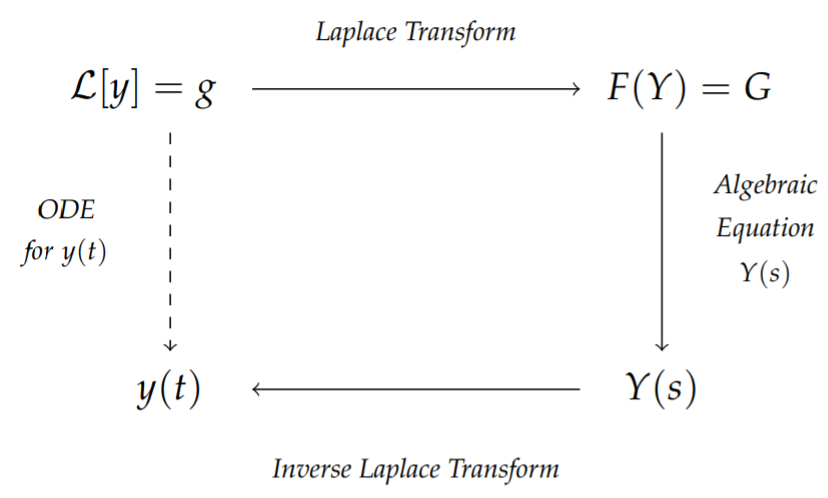
The general idea is that one transforms the equation for an unknown function \(y(t)\) into an algebraic equation for its transform, \(Y(t)\). Typically, the algebraic equation is easy to solve for \(Y(s)\) as a function of \(s\). Then, one transforms back into \(t\)-space using Laplace transform tables and the properties of Laplace transforms. The scheme is shown in Figure \(\PageIndex{1}\).
Solve the initial value problem \(y^{\prime}+3 y=e^{2 t}, y(0)=1\).
Solution
The first step is to perform a Laplace transform of the initial value problem. The transform of the left side of the equation is
\[\mathcal{L}\left[y^{\prime}+3 y\right]=s Y-y(0)+3 Y=(s+3) Y-1 .\nonumber \]
Transforming the right hand side, we have
\[\mathcal{L}\left[e^{2 t}\right]=\frac{1}{s-2}\nonumber \]
Combining these two results, we obtain
\[(s+3) Y-1=\frac{1}{s-2} \text {. }\nonumber \]
The next step is to solve for \(Y(s)\) :
\[Y(s)=\frac{1}{s+3}+\frac{1}{(s-2)(s+3)} .\nonumber \]
Now, we need to find the inverse Laplace transform. Namely, we need to figure out what function has a Laplace transform of the above form. We will use the tables of Laplace transform pairs. Later we will show that there are other methods for carrying out the Laplace transform inversion.
The inverse transform of the first term is \(e^{-3 t}\). However, we have not seen anything that looks like the second form in the table of transforms that we have compiled; but, we can rewrite the second term by using a partial fraction decomposition. Let’s recall how to do this.
The goal is to find constants, \(A\) and \(B\), such that
\[\frac{1}{(s-2)(s+3)}=\frac{A}{s-2}+\frac{B}{s+3} \text {. }\label{eq:6} \]
We picked this form because we know that recombining the two will have the same denominator. We just need to make sure the afterwards. So, adding the two terms, we have
\[\frac{1}{(s-2)(s+3)}=\frac{A(s+3)+B(s-2)}{(s-2)(s+3)} .\nonumber \]
Equating numerators,
\[1=A(s+3)+B(s-2) .\nonumber \]
There are several ways to proceed at this point.
This is an example of carrying out a partial fraction decomposition.
- Method 1.
We can rewrite the equation by gathering terms with common powers of \(s\), we have\[(A+B) s+3 A-2 B=1 .\nonumber \]
The only way that this can be true for all \(s\) is that the coefficients of the different powers of s agree on both sides. This leads to two equations for \(A\) and \(B\) :
\[\begin{array}{r} A+B=0 \\ 3 A-2 B=1 . \end{array}\label{eq:7} \]
The first equation gives \(A=-B\), so the second equation becomes \(-5 B=1\). The solution is then \(A=-B=\frac{1}{5}\).
- Method 2.
Since the equation \(\frac{1}{(s-2)(s+3)}=\frac{A}{s-2}+\frac{B}{s+3}\) is true for all \(s\), we can pick specific values. For \(s=2\), we find \(1=5 A\), or \(A=\frac{1}{5}\). For \(s=-3\), we find \(1=-5 B\), or \(B=-\frac{1}{5}\). Thus, we obtain the same result as Method 1, but much quicker. - Method 3.
We could just inspect the original partial fraction problem. Since the numerator has no \(s\) terms, we might guess the form\[\frac{1}{(s-2)(s+3)}=\frac{1}{s-2}-\frac{1}{s+3}.\nonumber \]
But, recombining the terms on the right hand side, we see that
\[\frac{1}{s-2}-\frac{1}{s+3}=\frac{5}{(s-2)(s+3)} \text {. }\nonumber \]
Since we were off by 5 , we divide the partial fractions by 5 to obtain
\[\frac{1}{(s-2)(s+3)}=\frac{1}{5}\left[\frac{1}{s-2}-\frac{1}{s+3}\right] \text {, }\nonumber \]
which once again gives the desired form.
Returning to the problem, we have found that
\[Y(s)=\frac{1}{s+3}+\frac{1}{5}\left(\frac{1}{s-2}-\frac{1}{s+3}\right) .\nonumber \]
We can now see that the function with this Laplace transform is given by
\[y(t)=\mathcal{L}^{-1}\left[\frac{1}{s+3}+\frac{1}{5}\left(\frac{1}{s-2}-\frac{1}{s+3}\right)\right]=e^{-3 t}+\frac{1}{5}\left(e^{2 t}-e^{-3 t}\right)\nonumber \]
works. Simplifying, we have the solution of the initial value problem
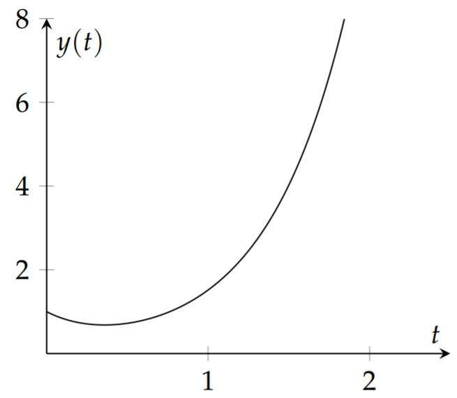
\[y(t)=\frac{1}{5} e^{2 t}+\frac{4}{5} e^{-3 t} .\nonumber \]
We can verify that we have solved the initial value problem.
\[y^{\prime}+3 y=\frac{2}{5} e^{2 t}-\frac{12}{5} e^{-3 t}+3\left(\frac{1}{5} e^{2 t}+\frac{4}{5} e^{-3 t}\right)=e^{2 t}\nonumber \]
and \(y(0)=\frac{1}{5}+\frac{4}{5}=1\).
Solve the initial value problem \(y^{\prime \prime}+4 y=0, y(0)=1, y^{\prime}(0)=3\).
Solution
We can probably solve this without Laplace transforms, but it is a simple exercise. Transforming the equation, we have
\[\begin{align} 0&=s^2Y-sy(0)-y'(0)+4Y\nonumber \\ &=(s^2+4)Y-s-3.\label{eq:8}\end{align} \]
Solving for \(Y\), we have
\[Y(s)=\frac{s+3}{s^2+4}.\nonumber \]
We now ask if we recognize the transform pair needed. The denominator looks like the type needed for the transform of a sine or cosine. We just need to play with the numerator. Splitting the expression into two terms, we have
\[Y(s)=\frac{s}{s^{2}+4}+\frac{3}{s^{2}+4} .\nonumber \]
The first term is now recognizable as the transform of \(\cos 2 t\). The second term is not the transform of \(\sin 2 t\). It would be if the numerator were a 2 . This can be corrected by multiplying and dividing by 2:
\[\frac{3}{s^{2}+4}=\frac{3}{2}\left(\frac{2}{s^{2}+4}\right) \text {. }\nonumber \]
The solution is then found as
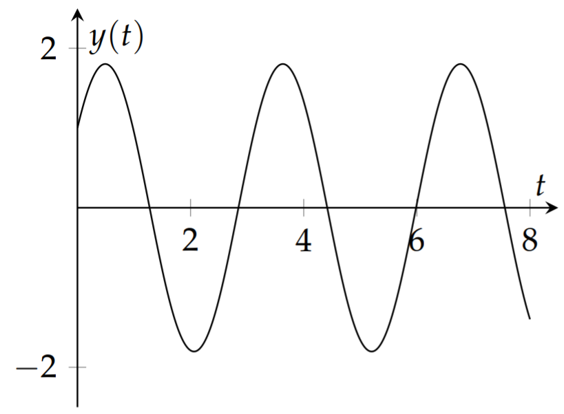
\[y(t)=\mathcal{L}^{-1}\left[\frac{s}{s^{2}+4}+\frac{3}{2}\left(\frac{2}{s^{2}+4}\right)\right]=\cos 2 t+\frac{3}{2} \sin 2 t .\nonumber \]
The reader can verify that this is the solution of the initial value problem.
Step and Impulse Functions
Often the initial value problems that one faces in differential equations courses can be solved using either the Method of Undetermined Coefficients or the Method of Variation of Parameters. However, using the latter can be messy and involves some skill with integration. Many circuit designs can be modeled with systems of differential equations using Kirchoff’s Rules. Such systems can get fairly complicated. However, Laplace transforms can be used to solve such systems and electrical engineers have long used such methods in circuit analysis.
In this section we add a couple of more transform pairs and transform properties that are useful in accounting for things like turning on a driving force, using periodic functions like a square wave, or introducing impulse forces.
We first recall the Heaviside step function, given by
\[H(t)= \begin{cases}0, & t<0, \\ 1, & t>0 .\end{cases}\label{eq:9} \]
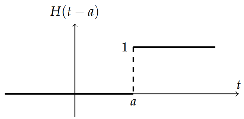
A more general version of the step function is the horizontally shifted step function, \(H(t-a)\). This function is shown in Figure \(\PageIndex{4}\). The Laplace transform of this function is found for \(a>0\) as
\[\begin{align} \mathcal{L}[H(t-a)] &=\int_{0}^{\infty} H(t-a) e^{-s t} d t\nonumber \\ &=\int_{a}^{\infty} e^{-s t} d t\nonumber \\ &=\left.\frac{e^{-s t}}{s}\right|_{a} ^{\infty}=\frac{e^{-a s}}{s} .\label{eq:10} \end{align} \]
Just like the Fourier transform, the Laplace transform has two shift theorems involving the multiplication of the function, \(f(t)\), or its transform, \(F(s)\), by exponentials. The first and second shifting properties/theorems are given by
\[\begin{align} \mathcal{L}\left[e^{a t} f(t)\right] &=F(s-a)\label{eq:11} \\ \mathcal{L}[f(t-a) H(t-a)] &=e^{-a s} F(s)\label{eq:12} \end{align} \]
We prove the First Shift Theorem and leave the other proof as an exercise for the reader. Namely,
\[\begin{align} \mathcal{L}\left[e^{a t} f(t)\right] &=\int_{0}^{\infty} e^{a t} f(t) e^{-s t} d t\nonumber \\ &=\int_{0}^{\infty} f(t) e^{-(s-a) t} d t=F(s-a) .\label{eq:13} \end{align} \]
Compute the Laplace transform of \(e^{-a t} \sin \omega t\).
Solution
This function arises as the solution of the underdamped harmonic oscillator. We first note that the exponential multiplies a sine function. The shift theorem tells us that we first need the transform of the sine function. So, for \(f(t)=\sin \omega t\), we have
\[F(s)=\frac{\omega}{s^{2}+\omega^{2}} .\nonumber \]
Using this transform, we can obtain the solution to this problem as
\[\mathcal{L}\left[e^{-a t} \sin \omega t\right]=F(s+a)=\frac{\omega}{(s+a)^{2}+\omega^{2}} .\nonumber \]
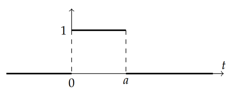
More interesting examples can be found using piecewise defined functions. First we consider the function \(H(t)-H(t-a)\). For \(t<0\) both terms are zero. In the interval \([0, a]\) the function \(H(t)=1\) and \(H(t-a)=0\). Therefore, \(H(t)-H(t-a)=1\) for \(t \in[0, a]\). Finally, for \(t>a\), both functions are one and therefore the difference is zero. The graph of \(H(t)-H(t-a)\) is shown in Figure \(\PageIndex{5}\).
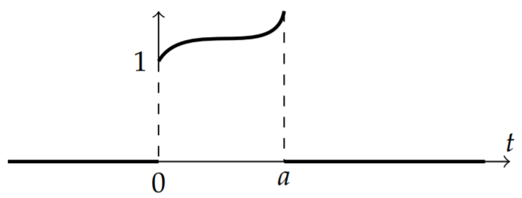
We now consider the piecewise defined function
\[g(t)=\left\{\begin{array}{cc} f(t), & 0 \leq t \leq a, \\ 0, & t<0, t>a . \end{array}\right.\nonumber \]
This function can be rewritten in terms of step functions. We only need to multiply \(f(t)\) by the above box function,
\[g(t)=f(t)[H(t)-H(t-a)]\nonumber \]
We depict this in Figure \(\PageIndex{6}\).
Even more complicated functions can be written in terms of step functions. We only need to look at sums of functions of the form \(f(t)[H(t-a)-H(t-b)]\) for \(b>a\). This is similar to a box function. It is nonzero between \(a\) and \(b\) has height \(f(t)\).
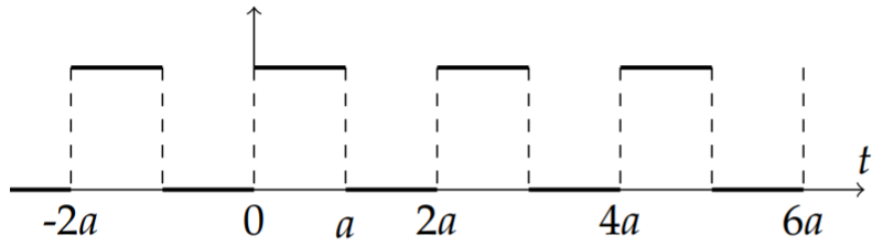
We show as an example the square wave function in Figure \(\PageIndex{7}\). It can be represented as a sum of an infinite number of boxes,
\[f(t)=\sum_{n=-\infty}^{\infty}[H(t-2 n a)-H(t-(2 n+1) a)],\nonumber \]
for \(a>0\).
Find the Laplace Transform of a square wave "turned on" at \(t=0 .\)
Solution
We let
\[f(t)=\sum_{n=0}^{\infty}[H(t-2 n a)-H(t-(2 n+1) a)], \quad a>0 .\nonumber \]
Using the properties of the Heaviside function, we have
\[\begin{align} \mathcal{L}[f(t)] &=\sum_{n=0}^{\infty}[\mathcal{L}[H(t-2 n a)]-\mathcal{L}[H(t-(2 n+1) a)]]\nonumber \\ &=\sum_{n=0}^{\infty}\left[\frac{e^{-2 n a s}}{s}-\frac{e^{-(2 n+1) a s}}{s}\right]\nonumber \\ &=\frac{1-e^{-a s}}{s} \sum_{n=0}^{\infty}\left(e^{-2 a s}\right)^{n}\nonumber \\ &=\frac{1-e^{-a s}}{s}\left(\frac{1}{1-e^{-2 a s}}\right)\nonumber \\ &=\frac{1-e^{-a s}}{s\left(1-e^{-2 a s}\right)}\label{eq:14} \end{align} \]
Note that the third line in the derivation is a geometric series. We summed this series to get the answer in a compact form since \(e^{-2 a s}<1\).
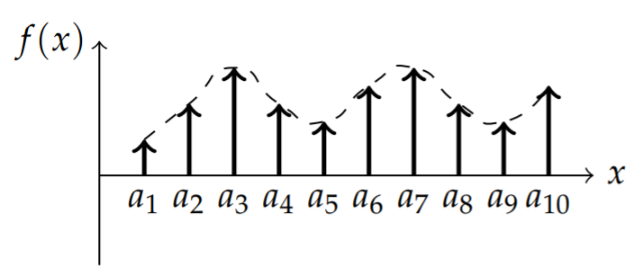
Other interesting examples are provided by the delta function. The Dirac delta function can be used to represent a unit impulse. Summing over a number of impulses, or point sources, we can describe a general function as shown in Figure \(\PageIndex{8}\). The sum of impulses located at points \(a_{i}, i=1, \ldots, n\) with strengths \(f\left(a_{i}\right)\) would be given by
\[f(x)=\sum_{i=1}^{n} f\left(a_{i}\right) \delta\left(x-a_{i}\right) .\nonumber \]
A continuous sum could be written as
\[f(x)=\int_{-\infty}^{\infty} f(\xi) \delta(x-\xi) d \xi .\nonumber \]
This is simply an application of the sifting property of the delta function. We will investigate a case when one would use a single impulse. While a mass on a spring is undergoing simple harmonic motion, we hit it for an instant at time \(t=a\). In such a case, we could represent the force as a multiple of \(\delta(t-a)\).
\(\mathcal{L}[\delta(t-a)]=e^{-a s} .\)
One would then need the Laplace transform of the delta function to solve the associated initial value problem. Inserting the delta function into the Laplace transform, we find that for \(a>0\)
\[\begin{align} \mathcal{L}[\delta(t-a)] &=\int_{0}^{\infty} \delta(t-a) e^{-s t} d t\nonumber \\ &=\int_{-\infty}^{\infty} \delta(t-a) e^{-s t} d t\nonumber \\ &=e^{-a s} .\label{eq:15} \end{align} \]
Solve the initial value problem \(y^{\prime \prime}+4 \pi^{2} y=\delta(t-2), y(0)=\) \(y^{\prime}(0)=0\).
Solution
This initial value problem models a spring oscillation with an impulse force. Without the forcing term, given by the delta function, this spring is initially at rest and not stretched. The delta function models a unit impulse at \(t=2\). Of course, we anticipate that at this time the spring will begin to oscillate. We will solve this problem using Laplace transforms.
First, we transform the differential equation:
\[s^{2} Y-s y(0)-y^{\prime}(0)+4 \pi^{2} Y=e^{-2 s} .\nonumber \]
Inserting the initial conditions, we have
\[\left(s^{2}+4 \pi^{2}\right) Y=e^{-2 s} \text {. }\nonumber \]
Solving for \(Y(s)\), we obtain
\[Y(s)=\frac{e^{-2 s}}{s^{2}+4 \pi^{2}} .\nonumber \]
We now seek the function for which this is the Laplace transform. The form of this function is an exponential times some Laplace transform, \(F(s)\). Thus, we need the Second Shift Theorem since the solution is of the form \(Y(s)=e^{-2 s} F(s)\) for
\[F(s)=\frac{1}{s^{2}+4 \pi^{2}} .\nonumber \]
We need to find the corresponding \(f(t)\) of the Laplace transform pair. The denominator in \(F(s)\) suggests a sine or cosine. Since the numerator is constant, we pick sine. From the tables of transforms, we have
\[\mathcal{L}[\sin 2 \pi t]=\frac{2 \pi}{s^{2}+4 \pi^{2}} .\nonumber \]
So, we write
\[F(s)=\frac{1}{2 \pi} \frac{2 \pi}{s^{2}+4 \pi^{2}} .\nonumber \]
This gives \(f(t)=(2 \pi)^{-1} \sin 2 \pi t\).
We now apply the Second Shift Theorem, \(\mathcal{L}[f(t-a) H(t-a)]=e^{-a s} F(s)\), or
\[\begin{align}y(t)&=\mathcal{L}^{-1}\left[e^{-2s}F(s)\right]\nonumber \\ &=H(t-2)f(t-2)\nonumber \\ &=\frac{1}{2\pi}H(t-2)\sin 2\pi (t-2).\label{eq:16}\end{align} \]
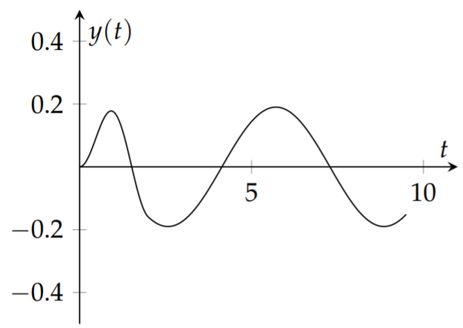
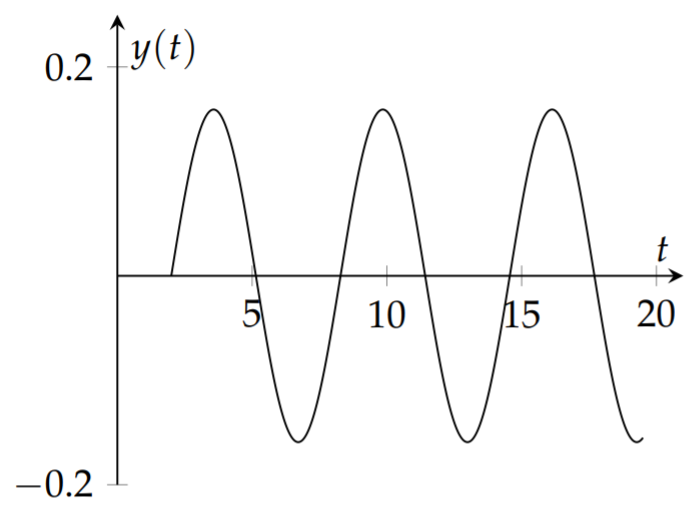
This solution tells us that the mass is at rest until \(t = 2\) and then begins to oscillate at its natural frequency. A plot of this solution is shown in Figure \(\PageIndex{9}\).
Solve the initial value problem
\[y^{\prime \prime}+y=f(t), \quad y(0)=0, y^{\prime}(0)=0,\nonumber \]
where
\[f(t)=\left\{\begin{array}{cl} \cos \pi t, & 0 \leq t \leq 2, \\ 0, & \text { otherwise. } \end{array}\right.\nonumber \]
Solution
We need the Laplace transform of \(f(t)\). This function can be written in terms of a Heaviside function, \(f(t)=\cos \pi t H(t-2)\). In order to apply the Second Shift Theorem, we need a shifted version of the cosine function. We find the shifted version by noting that \(\cos \pi(t-2)=\cos \pi t\). Thus, we have
\[\begin{align} f(t) &=\cos \pi t[H(t)-H(t-2)]\nonumber \\ &=\cos \pi t-\cos \pi(t-2) H(t-2), \quad t \geq 0 .\label{eq:17} \end{align} \]
The Laplace transform of this driving term is
\[F(s)=\left(1-e^{-2 s}\right) \mathcal{L}[\cos \pi t]=\left(1-e^{-2 s}\right) \frac{s}{s^{2}+\pi^{2}} .\nonumber \]
Now we can proceed to solve the initial value problem. The Laplace transform of the initial value problem yields
\[\left(s^{2}+1\right) Y(s)=\left(1-e^{-2 s}\right) \frac{s}{s^{2}+\pi^{2}} .\nonumber \]
Therefore,
\[Y(s)=\left(1-e^{-2 s}\right) \frac{s}{\left(s^{2}+\pi^{2}\right)\left(s^{2}+1\right)} .\nonumber \]
We can retrieve the solution to the initial value problem using the Second Shift Theorem. The solution is of the form \(Y(s)=\left(1-e^{-2 s}\right) G(s)\) for
\[G(s)=\frac{s}{\left(s^{2}+\pi^{2}\right)\left(s^{2}+1\right)} .\nonumber \]
Then, the final solution takes the form
\[y(t)=g(t)-g(t-2) H(t-2) .\nonumber \]
We only need to find \(g(t)\) in order to finish the problem. This is easily done by using the partial fraction decomposition
\[G(s)=\frac{s}{\left(s^{2}+\pi^{2}\right)\left(s^{2}+1\right)}=\frac{1}{\pi^{2}-1}\left[\frac{s}{s^{2}+1}-\frac{s}{s^{2}+\pi^{2}}\right] .\nonumber \]
Then,
\[g(t)=\mathcal{L}^{-1}\left[\frac{s}{\left(s^{2}+\pi^{2}\right)\left(s^{2}+1\right)}\right]=\frac{1}{\pi^{2}-1}(\cos t-\cos \pi t) .\nonumber \]
The final solution is then given by
\[y(t)=\frac{1}{\pi^{2}-1}[\cos t-\cos \pi t-H(t-2)(\cos (t-2)-\cos \pi t)] .\nonumber \]
A plot of this solution is shown in Figure \(\PageIndex{10}\).