1.7: Symplectic integrators

Symplectic integrators

Energy conserving ODEs

The ODE solvers examined thus far are meant for general purpose applications. However, these is a special set of ODEs which are not well served by the general purpose methods. Those are ODEs which describe mechanical systems undergoing lossless motion. "Lossless" means the system does not dissipate energy. Some examples are:

• The frictionless simple harmonic oscillator, which we have seen many times already.
• The frictionless hanging pendulum.
• Motion of planets or satellites in space.

You might regard the first two examples as oversimple models. However, a pendulum swinging in a vacuum is very close to lossless. The LIGO apparatus which detected gravitational waves used pendulums hanging in a vacuum as part of its operation, so the (almost) frictionless pendulum is a physical reality. Also, the motion of objects in space occurs with almost no dissipation – there is no atmosphere to provide resistance to motion. Accurately simulating their motion requires ODE solvers which respect the fact they experience no friction when moving – they don’t dissipate any energy. Unfortunately, the problem with ODE solvers studied so far is that none of them conserve energy. If you want to calculate the trajectory a rocket must travel in order to dock with the orbiting space station, it’s crucial that your ODE solver calculates the trajectory perfectly, and that means it needs compute trajectories which are energy conserving.

What is energy? In a physics class you probably learned that energy is something which is conserved. But what does that mean? And why is kinetic energy \((1/2) m v^2\)? What is going on, mathematically?

For some insights we once again turn to the simple harmonic oscillator, \[\tag{eq:7.1} m \frac{d^2 y}{d t^2} = -k y\] Associated with this equation is a so-called energy, \[\tag{eq:7.2} E = \frac{1}{2} m \left( \frac{d y}{d t} \right)^2 + \frac{1}{2} k y^2\] which is a function of the variables position \(y\) and velocity \(dy/dt\). From your physics class you may recognize the term on the left as the "kinetic energy" and the term on the right as the "potential energy" of the SHO. The important property of this energy definition is that any solution \(y(t)\) of the ODE [eq:7.1] will automatically conserve the energy function [eq:7.2]. "Conserve" means that the energy \(E\) will remain constant for all times. This can be shown by considering the time derivative of \(E\). \[\frac{d E}{d t} = m \left( \frac{d y}{d t} \right)\left( \frac{d^2 y}{d t^2} \right) + k y \left( \frac{d y}{d t} \right) \tag{eq:7.3}\] then substitute the value of \(m (d^2 y/d t^2)\) from [eq:7.1] into this equation to get

\[\frac{d E}{d t} = -k y \left( \frac{d y}{d t} \right) + k y \left( \frac{d y}{d t} \right) \tag{eq:7.4}\]

\[ = 0 \tag{7.5}\]

This says that \(E\) never changes – it is conserved by any solution to [eq:7.1]. In general, some – but not all – ODEs admit an energy which is conserved. The exact form of the energy depends upon the ODE under consideration. But if a conserved energy exists for a particular ODE, then a good solver should produce solutions which conserve energy. Unfortunately, most solvers don’t. We have seen this several times through the course of this booklet – see 2.9, 3.5, 4.5, and 4.13. Those figures all show the amplitude of the oscillation growing or shrinking with increasing time – behavior which evidences the energy is changing with time.

There is a class of solvers which do conserve energy. They fall under the rubric "symplectic integrators". The reason they have this name has to do with Hamiltonian mechanics, a generalization of Newtonian mechanics which we will touch on in 7.4. Symplectic integrators are used only for second-degree ODEs such as found in Newton’s second law. Consequently, they are very important for calculating the motion of objects in space, including planets, spacecraft, comets, and so on. They come in many orders of accuracy, similar to the other solvers discussed in this booklet. I will only discuss the simplest method – symplectic Euler – here since this symplectic integrators are a specialized subject and it’s enough to simply see the concepts rather than review the entire field.

Symplectic Euler

As mentioned above, symplectic integrators are used to solve second-degree ODEs.l That means the integrators are applied to a system of two 1st-degree ODEs. That is, we start with teh system to solve \[\begin{aligned} \frac{d u}{d t} =& f(t, v) \\ \frac{d v}{d t} =& g(t, u) \end{aligned} \tag{eq:7.6}\] With this definition, here is symplectic Euler: \[\begin{aligned} v_{n+1} =& v_n + h g(t_n, u_n) \\ u_{n+1} =& u_n + h f(t_n, v_{n+1}) \end{aligned} \tag{eq:7.7}\] Note that first \(v\) is updated, then \(u\) us updated using the already updated \(v\). The method is symmetric with respect to which is updated first,, so you can also use \[\begin{aligned} u_{n+1} =& u_n + h f(t_n, v_{n}) v_{n+1} =& v_n + h g(t_n, u_n+1) \\ \end{aligned} \tag{eq:7.8}\] This is sometimes called a semi-implicit method (or semi-implicit Euler scheme) since the updated value \(v_{n+1}\) (or \(u_{n+1}\))is used in the middle of the full two-step computation.

Example: the simple harmonic oscillator

We know the analytical solutions of the simple harmonic oscillator equation [eq:7.1] conserve energy. Now we will see if the solution produced by symplectic Euler also conserves energy. For the RHS of [eq:7.6] we have \[\begin{aligned} \nonumber f(t, v) =& -\omega^2 v \\ \nonumber g(t, u) =& u\end{aligned}\] using the usual definition \(\omega^2 = k/m\). Inserting these into [eq:7.8] yields \[\begin{aligned} v_{n+1} =& v_n + h u_n \\ u_{n+1} =& u_n - h \omega^2 v_{n+1} \end{aligned} \tag{eq:7.9}\] We could implement this system on the computer as it stands, but for the purposes of stability analysis we will convert it into a matrix propagator form. To do so move the future to the LHS and the present to the RHS. We get \[\nonumber \begin{aligned} u_{n+1} + h \omega^2 v_{n+1} =& u_n \\ v_{n+1} =& v_n + h u_n \end{aligned}\]

Now write both sides as matrix-vector products. We get \[\nonumber \begin{pmatrix} 1 & h \omega^2 \\ 0 & 1 \end{pmatrix} \begin{pmatrix} u_{n+1} \\ v_{n+1} \end{pmatrix} = \begin{pmatrix} 1 & 0 \\ h & 1 \end{pmatrix} \begin{pmatrix} u_{n} \\ v_{n} \end{pmatrix}\] Now move the LHS matrix to the RHS \[\nonumber \begin{pmatrix} u_{n+1} \\ v_{n+1} \end{pmatrix} = \begin{pmatrix} 1 & h \omega^2 \\ 0 & 1 \end{pmatrix}^{-1} \begin{pmatrix} 1 & 0 \\ h & 1 \end{pmatrix} \begin{pmatrix} u_{n} \\ v_{n} \end{pmatrix}\] Simplifying, this becomes \[\begin{pmatrix} u_{n+1} \\ v_{n+1} \end{pmatrix} = \begin{pmatrix} 1 - h^2 \omega^2& -h \omega^2 \\ h & 1 \end{pmatrix} \begin{pmatrix} u_{n} \\ v_{n} \end{pmatrix} \tag{eq:7.10}\]

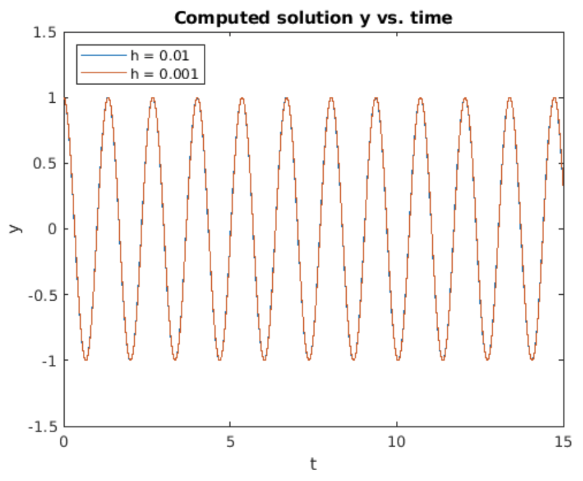
This defines an iteration method using the matrix as a propagator. Note the similarity to the forward Euler propagation matrix [eq:2.19]: only the (1,1) element is different. The results of implementing this iteration are shown in 7.1. Unlike the cases of forward and backward Euler, this method evidences no growth nor decay of the oscillation amplitude with time.

Figure 7.1: The simple harmonic oscillator integrated using symplectic Euler. Note the longer time span than plotted for previous solutions of the SHO. No growth nor decay of the oscillation is evident in this plot – the energy of the solution is conserved by the method, at least at this scale.

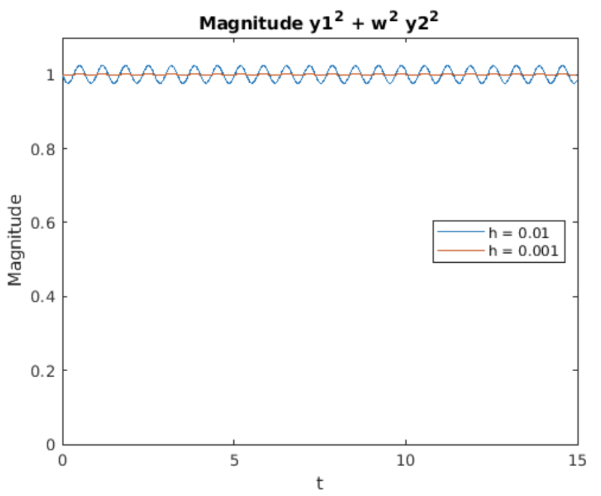
Energy conservation is also shown in 7.2 which plots \(u(t)^2 + \omega^2 v(t)^2\). In analogy to \(\sin^2(t) + cos^2(t) = 1\), the energy \(u(t)^2 + \omega^2 v(t)^2\) should remain constant. It does, except it evinces little wiggles which depend upon time. Note that the average value remains equal to one.

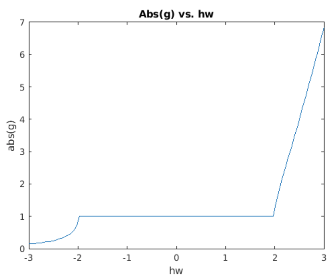
Of course, now the question is why does symplectic Euler conserve energy? As usual, the answer lies in computing the eigenvalues of the propagator matrix. Call \(g\) the eigenvalue (again, for "growth factor"). The eigenvalue equation is then \[\nonumber det \begin{pmatrix} 1 - h^2 \omega^2 - g & -h \omega^2 \\ h & 1 - g \end{pmatrix} = 0\] Solving for \(g\) gives \[\tag{eq:7.11} g = 1 - \frac{h^2 \omega^2}{2} \pm \frac{h \omega \sqrt{h^2 \omega^2 - 4}}{2}\] This is a nasty expression at first glance. However, our goal is to see if \(|g| = 1\) for any values of \(h \omega\). If \(|g| = 1\) then we have a method which does not cause the solution amplitude to grow or decay. Therefore, an easy way to understand [eq:7.11] is to simply use Matlab to plot \(|g|\) vs. \(h \omega\). This is shown in 7.3. We see that \(|g| = 1\) when \(|h \omega| < 2\). Therefore, symplectic Euler method maintains the amplitude of the simple harmonic oscillator – that is, it conserves energy.

Figure 7.2: A plot of \(u(t)^2 + \omega^2 v(t)^2\) which shows symplectic Euler conserves energy on average. Note that the amplitude remains close to one over the entire simulation time. It wiggles up and down but does not grow nor shrink over a longer time scale.

Knowing that \(|g| = 1\) when \(|h \omega| < 2\) allows us to take a few additional easy analytic steps. When \(|h \omega| < 2\) the rightmost term in [eq:7.11] is pure imaginary while the other two terms are real. That means we can compute \(|g|^2 = \Re(g)^2 + \Im(g)^2\), \[\nonumber |g|^2 = \left(1 - \frac{h^2 \omega^2}{2}\right)^2 + \left( \frac{h \omega \sqrt{4 - h^2 \omega^2}}{2} \right)^2\] \[\nonumber = \left(1 - h^2 \omega^2 + \left( \frac{h^2 \omega^2}{2} \right)^2 \right) + \left( \frac{h^2 \omega^2 (4 - h^2 \omega^2)}{4} \right)\] \[\nonumber = 1\] as was found in the plot 7.3. This confirms our numerical observation in 7.3 that \(|g| = 1\). Outside this range, the growth factor is not one, meaning that symplectic Euler doesn’t conserve energy outside of the range \(|h \omega| < 2\). However, this is not a big limitation since one generally needs \(h \ll 1/\omega\) to compute smooth oscillations. That is, you need to sample at least a couple of points inside each oscillation in order to simulate it accurately, so achieving \(|h \omega| < 2\) is compatible with choosing a good step size.

Figure 7.3: The growth factor \(|g|\) plotted vs. \(h \omega\). The growth factor is exactly one when \(|h \omega| < 2\). Therefore, in this range the symplectic Euler method maintains the amplitude of the simple harmonic oscillator – that is, it conserves energy. However, the plots walk away from each other in time depending upon the value of \(h\).

Conservative systems, phase space, and Liouville’s theorem

This section is a brief detour into the physics of energy conservation in classical mechanics. At the beginning of 7 above I mentioned that some, but not all ODEs have an accompanying energy. In advanced mechanics, the equations of motion of a system which conserves energy are found by first writing down a so-called "Hamiltonian", and then deriving the position and momentum of all particles in the system from the Hamiltonian. The Hamiltonian is a scalar function which plays the role of the energy of the system, but is written in terms of position and momentum variables. For the SHO, the Hamiltonian is \[\tag{eq:7.12} H(p,x) = \frac{p^2}{2 m} + \frac{1}{2} k x^2\] where \(p\) is the momentum of the oscillator and \(x\) is its position. Note this is the same as the total energy [eq:7.2] where we have replaced the kinetic energy written in terms of the velocity \(m v^2 / 2\) with the equivalent expression written in terms of momentum, \(p^2/2 m\). Then, to get the equations of motion of the system, the Hamiltonian formalism says they are found from Hamilton’s equations, \[\tag{eq:7.13} \frac{d x}{d t} = \frac{\partial H}{ \partial p}\] \[\tag{eq:7.14} \frac{d p}{d t} = -\frac{\partial H}{ \partial x}\] In the case of the SHO we use the Hamiltonian [eq:7.12] and these equations to get the equations of motion of the oscillator, \[\nonumber \frac{d x}{d t} = \frac{p}{m}\] \[\nonumber \frac{d p}{d t} = -k x\] This pair of equations should remind you strongly of those introduced back in [eq:2.17] – they’re the same equations but written in terms of position and momentum instead of position and velocity. In Hamiltonian mechanics, you first use physical reasoning to construct and write down a Hamiltonian. Then you derive the equations of motion from the Hamiltonian using these equations. The point is that Hamiltonian mechanics gives you a general, step-by-step procedure to derive the equations of motion of any system. By contrast, Newtonian mechanics relies on ad-hoc arguments about forces and accelerations to derive the equations of motion, and every system is handled differently depending upon its physical configuration.

Since the Hamiltonian is the energy function of the system, it is conserved as long as time does not appear explicitly in its formula. This is clearly the case for the SHO Hamiltonian, [eq:7.12]. At a deep level, energy conservation is a consequence of Noether’s theorem, which says that every symmetry of the Hamiltonian implies a corresponding conserved quantity. For the SHO Hamiltonian, we may replace time \(t\) with \(t + \tau\), where \(\tau\) represents a constant shift of the time axis. Upon making this replacement \(t \rightarrow t + \tau\), the form of the Hamiltonian remains the same. That is, this Hamiltonian is invariant with respect to the transformation \(t \rightarrow t + \tau\). Another way to say it is that the Hamiltonian is symmetric with respect to time shifts. As a consequence of Noether’s theorem, this symmetry implies an associated quantity is conserved, and in this case the conserved quantity is the energy. This should answer the question posed back in 7.1, why is energy conserved for the SHO? Energy is conserved by the SHO because its Hamiltonian has time-shift symmetry! Noether’s theorem is very profound and is used by physicists to reason about many different conserved quantities like electric charge, mass, parity, and other quantities. Unfortunately, while it is very interesting, further discussion of Noether’s theorem is far outside the scope of this booklet.

Another important result from classical mechanics is that any system derived from a time-invariant Hamiltonian will conserve volumes in phase space. What does this mean?

• First, phase space is defined as the space of all possible states of the system. For example, a body undergoing one-dimensional motion has a two-dimensional phase space: the set of all possible positions and momenta, \([x, p]\) without regard for any equations of motion. (Equations of motion will be imposed later and will naturally restrict the set of possible \([x, p]\) to orbits within the full phase space.)
• Once the phase space is defined, any particular mechanical system may be described via a Hamiltonian defined on the phase space. Different mechanical systems will be described by different Hamiltonians. For example, the SHO has Hamiltonian \(H = p^2/2m + k x^2/2\) while the hanging pendulum has Hamiltonian \(H = p^2/2m + m g \cos(\theta)/2\).
• A time-invariant Hamiltonian is one which has no explicit dependence on time – the variable \(t\) does not appear in its formula. This is obviously the case for the SHO Hamiltonian [eq:7.12].
• The equations of motion derived from the Hamiltonian will define how any particular point \([x(t),p(t)]\) will evolve in time. You can visualize the evolution of a single point as a trajectory moving through phase space.
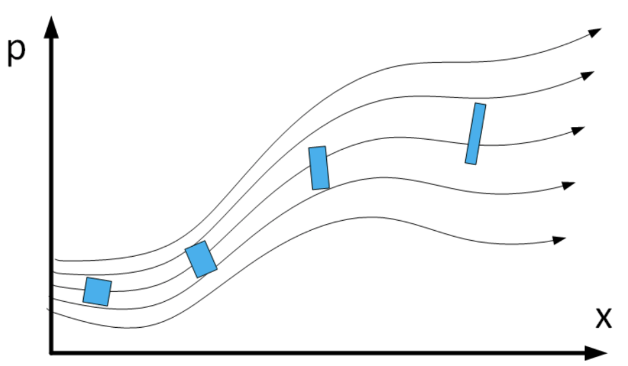
• Next consider a small region of phase space surrounding the initial phase-space point \([x(0),p(0)]\). See 7.4. Now ask, what happens to the volume of the region as time moves forward. Louiville’s theorem says that the volume \(V\) remains constant as the system evolves. That is, the blue region shown in the figure may twist and deform, but its volume will remain the same for all time.

Figure 7.4: Liouville’s theorem says that phase space volumes remain the same size when the system evolves under the action of a (time invariant) Hamiltonian.

A general proof of Liouville’s theorem is more difficult than I can explain in this booklet. But I will demonstrate that \([p(t), x(t)]^T\) trajectories generated by the SHO Hamiltonian conserve phase space volumes, and you can use my demonstration as motivation for accepting the general theorem.

Before examining the SHO, I want to start by considering what it means to measure volumes in phase space. I also give a criterion for recognizing when volume is conserved under a transformation. I will use a very simple picture to convey these ideas. Consider the case of a small square in a two-dimensional phase space. Take the sides of the square to be defined by two vectors, \(u\) and \(v\). Now consider what happens to \(u\) and \(v\) under a linear transform. "Linear transform" means matrix-vector multiplication. Under action of a \(2 \times 2\) matrix \(T\), we have \[\begin{pmatrix} u' \\ v' \end{pmatrix} = T \begin{pmatrix} u \\ v \end{pmatrix} \tag{eq:7.15}\] We think of \([u', v']^T\) as the output of the transformation, and \(T\) is the thing doing the transformation.

In your previous linear algebra class you probably learned that applying a linear transform to a vector produced a stretched and rotated copy of the input vector. If you’re lucky you may have seen that applying a linear transform to a square (whose sides are defined by two vectors) produced a parallelpiped output. This is shown in 7.5.

Figure 7.5: The action of the linear transform (matrix) \(T\) on vectors \(u\) and \(v\). In each case, the transformed result \(T u\) and \(T v\) is a stretched and rotated copy of the original vector. The initial square formed by \(u\) and \(v\) is thereby transformed into a parallelpiped.

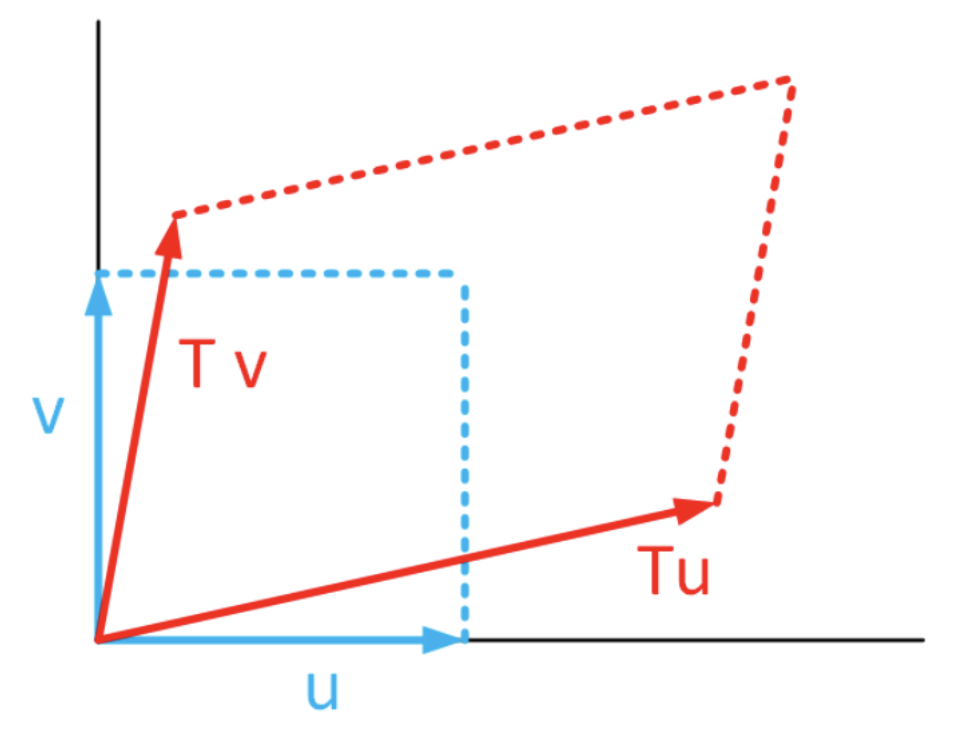
Now how to compute the volume (or area when working in 2D) of these shapes? Recall that the area subtended by the two vectors may be found using the determinant formula, \[\begin{aligned} A &= \begin{vmatrix} u_1 & u_2 \\ v_1 & v_2 \end{vmatrix} \\ &= u_1 v_2 - u_2 v_1 \end{aligned} \tag{eq:7.16}\] where we use the components of the vectors, \(u = [u_1, u_2]^T\) and \(v = [v_1, v_2]^T\). Another way to write this is using a quadratic form \[\tag{eq:7.17} A = \begin{pmatrix} u_1 & u_2 \\ \end{pmatrix} \begin{pmatrix} 0 & 1 \\ -1 & 0 \end{pmatrix} \begin{pmatrix} v_1 \\ v_2 \end{pmatrix} = u_1 v_2 - u_2 v_1\] You can easily see [eq:7.16] and [eq:7.17] give the same result by inspection. Due to its importance, we will give the matrix the name \(J\), so \[\nonumber J = \begin{pmatrix} 0 & 1 \\ -1 & 0 \end{pmatrix} \\\]

Now consider what it means for a transformation \(T\) to preserve volume. To preserve area we require that input area equals output area, \[\begin{aligned} \nonumber u^T J v &= u'^T J v' \\ \nonumber &= u^T T^T J T v\end{aligned}\] or we can drop the \(u\) and \(v\) and focus on the transformation itself. This equation requires the transformation obey \[\tag{eq:7.18} J = T^T J T\] A linear transform (matrix) which obeys [eq:7.18] is called "symplectic". If a transform \(T\) is symplectic, that means it preserves volumes.

We just looked at a symplectic linear transform. But what about the case of a general transform? And what does this have to do with Hamiltonians, energy conservation, and ODEs? Let’s again write down the SHO Hamiltonian, this time in non-dimensional form. (I don’t want to try to explain away the mass and stiffness constants in the below discussion – they would only make matters complicated.) The Hamiltonian is \[\tag{eq:7.19} H = \dfrac{1}{2}p^2 + \dfrac{1}{2} x^2\] Because time does not appear explicitly in this Hamiltonian, the system it describes will conserve energy. Now consider the motion of a point \([p, x]^T\) in the phase space governed by this Hamiltonian. The equations of motion obeyed by the point are \[\tag{eq:7.20} \dfrac{d}{dt} \begin{pmatrix} p \\ x \end{pmatrix} = \begin{pmatrix} -\partial H / \partial x \\ \partial H / \partial p \end{pmatrix}\] Next consider the trajectory of a point displaced from \([p, x]^T\) by \([\Delta p, \Delta x]^T\). We imagine these are the sides of the little volume we want to track. The displaced point’s motion is given by \[\nonumber \frac{d}{dt} \begin{pmatrix} p + \Delta p \\ x + \Delta x \end{pmatrix} = \begin{pmatrix} -\partial H / \partial x \\ \partial H / \partial p \end{pmatrix}\] Assuming \([\Delta p, \Delta x]^T\) are both small, we can approximate the motion using a Taylor series expansion, \[\tag{eq:7.21} \dfrac{d}{dt} \begin{pmatrix} p + \Delta p \\ x + \Delta x \end{pmatrix} \approx \left. \begin{pmatrix} -\partial H / \partial x \\ \partial H / \partial p \end{pmatrix} \right|_{p,x} + \left. \begin{pmatrix} -\partial^2 H / \partial x \partial p \\ \partial^2 H / \partial p^2 \end{pmatrix} \right|_{p,x} \Delta p + \left. \begin{pmatrix} -\partial^2 H / \partial x^2 \\ \partial^2 H / \partial p \partial x \end{pmatrix} \right|_{p,x} \Delta x\] Now subtract [eq:7.20] from [eq:7.21], and use the common notation for partial derivatives to get an expression for the evolution of the sides of the little volume, \[\nonumber \frac{d}{dt} \begin{pmatrix} \Delta p \\ \Delta x \end{pmatrix} \approx \left. \begin{pmatrix} -H_{xp} & -H_{xx} \\ H_{pp} & H_{px} \end{pmatrix} \right|_{p,x} \begin{pmatrix} \Delta p \\ \Delta x \end{pmatrix}\] This equation says that the change in the sides of the initial square is driven by the matrix of partial derivatives. That is, the partial derivative matrix plays the role of the transformation matrix \(A\) in [eq:7.17]. Therefore, we can say that the volume of the square remains constant under evolution if the symplicity condition [eq:7.18] holds. That is, to conserve phase space volumes, we want the following condition to hold for the SHO Hamiltonian: \[\begin{pmatrix} 0 & 1 \\ -1 & 0 \end{pmatrix} = \begin{pmatrix} -H_{xp} & H_{pp} \\ -H_{xx} & H_{px} \end{pmatrix} \begin{pmatrix} 0 & 1 \\ -1 & 0 \end{pmatrix} \begin{pmatrix} -H_{xp} & -H_{xx} \\ H_{pp} & H_{px} \end{pmatrix} \tag{eq:7.22}\] For the SHO Hamiltonian we have \[\begin{aligned} \nonumber H_{xx} &= \frac{\partial^2 H}{\partial x^2} = 1 \\ \nonumber H_{pp} &= \frac{\partial^2 H}{\partial p^2} = 1 \\ \nonumber H_{xp} &= H_{px} = 0\end{aligned}\] Upon inserting these values into [eq:7.22] and evaluating, we get \[\begin{aligned} \nonumber &\phantom{=i} \begin{pmatrix} 0 & 1 \\ -1 & 0 \end{pmatrix} \begin{pmatrix} 0 & 1 \\ -1 & 0 \end{pmatrix} \begin{pmatrix} 0 & -1 \\ 1 & 0 \end{pmatrix} \\ \nonumber &= \begin{pmatrix} 0 & 1 \\ -1 & 0 \end{pmatrix} \begin{pmatrix} 1 & 0 \\ 0 & 1 \end{pmatrix} \\ \nonumber &= \begin{pmatrix} 0 & 1 \\ -1 & 0 \end{pmatrix} \\ \nonumber &= J\end{aligned}\] Therefore, the transformation matrix induced by the SHO Hamiltonian is symplectic. And since it is symplectic, the transformation [eq:7.21] will preserve phase space volumes as promised.

Euler methods and conservation of phase space volumes

We end this booklet by looking at forward Euler and symplectic Euler and asking if one or both conserve phase space volumes. I wrote Matlab programs which draw a rectangle in phase space, then evolve the points in the rectangle using forward Euler and symplectic Euler for four oscillation periods.

(a) Forward Euler – zoomed out. The area under study starts as the rectangle at the 12 o’clock (top) of the circle. Four oscillation periods later, the rectangle has obviously grown in size – phase space area is not conserved.

(b) Forward Euler – zoomed in.

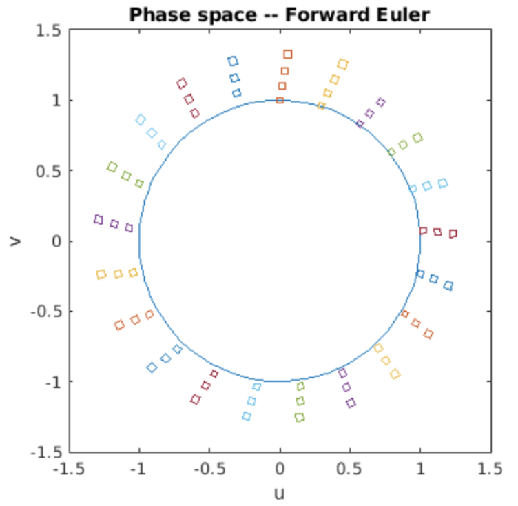
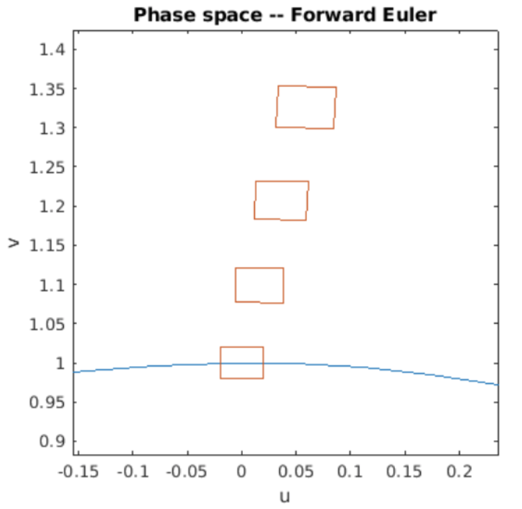
Figure 7.6: Phase space volumes evolved by forward Euler.

(a) Symplectic Euler – zoomed out. The area under study starts as the rectangle at the 12 o’clock (top) of the circle. Four oscillation periods later the rectangle has not grown in size, nor has it left the circle. The method is both stable and energy conserving.

(b) Symplectic Euler – zoomed in.

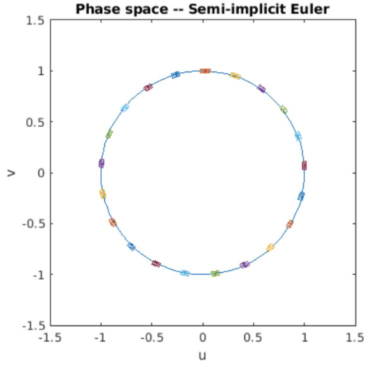
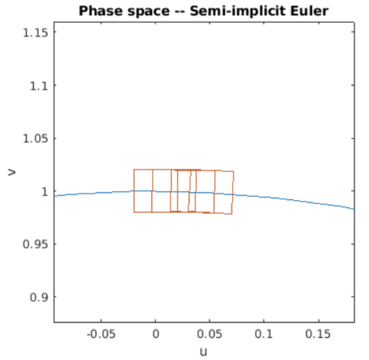
Figure 7.7: Phase space volumes evolved by symplectic Euler.

The program takes a snapshot of the rectangle multiple times during its evolution, and plots the rectanges on the circle of constant energy. The simulation results are shown in [fig:7.6] and [fig:7.7]. The results are clear: for the SHO, forward Euler is neither stable, nor does it conserve phase space volumes. However, symplectic Euler is both stable and also conserves phase space volumes as evidenced by the two plots.

Chapter summary

Here are the important points made in this chapter:

• General purpose ODE integrators usually don’t conserve energy. Therefore, they are inappropriate for problems where energy conservation is important, such as simulation of motion in space.
• Symplectic integrators are specialty solvers used for exactly those situations where it’s important that the ODE solver ensure conservation of energy. They are particularly common in computing the trajectories of objects in space.
• Energy conservation in mechanical systems is best understood in the context of Hamiltonian mechanics, which is a generalization of the Newtonian mechanics you probably learned about in your introductory physics classes.
• Besides conserving energy, a symplectic system also conserves phase space volumes. This fact is known as "Liouville’s theorem". A symplectic integrator will conserve phase space volumes as we demonstrated for the SHO – both via analytic methods as well as simulation using the symplectic Euler method.