
9.1: Bifurcation of Equilibria II
- Page ID
- 24186

We have examined fixed points of one dimensional autonomous vector fields where the matrix associated with the linearization of the vector field about the fixed point has a zero eigenvalue. It is natural to ask "are there more complicated bifurcations, and what makes them complicated?"
If one thinks about the examples considered so far, there are two possibilities that could complicate the situation. One is that there could be more than one eigenvalue of the linearization about the fixed point with zero real part (which would necessarily require a consideration of higher dimensional vector fields), and the other would be more complicated nonlinearity (or a combination of these two). Understanding how dimensionality and nonlinearity contribute to the "complexity" of a bifurcation (and what that might mean) is a very interesting topic, but beyond the scope of this course. This is generally a topic explored in graduate level courses on dynamical systems theory that emphasize bifurcation theory. Here we are mainly just introducing the basic ideas and issues with examples that one might encounter in applications. Towards that end we will consider an example of a bifurcation that is very important in applications–the Poincaré-Andronov-Hopf bifurcation (or just Hopf bifurcation as it is more commonly referred to). This is a bifurcation of a fixed point of an autonomous vector field where the fixed point is nonhyperbolic as a result of the Jacobian having a pair of purely imaginary eigenvalues, \(\pm i \mathcal{w}, \mathcal{w} \ne 0\). Therefore this type of bifurcation requires (at least two dimensions), and it is not characterize by a change in the number of fixed points, but by the creation of time dependent periodic solutions. We will analyze this situation by considering a specific example. References solely devoted to the Hopf bifurcation are the books of Marsden and McCracken and Hassard, Kazarinoff, and Wan.
We consider the following nonlinear autonomous vector field on the plane:
\[ \begin{align} \dot{x} &= \mu x- \mathcal{w}y+(ax-by)(x^2+y^2) \\[4pt] \dot{y} &= \mathcal{w}x+\mu y+(bx+ay)(x^2+y^2), (x, y) \in \mathbb{R}^2, \label{9.1} \end{align}\]
where we consider \(a\), \(b\), \(\mathcal{w}\) as fixed constants and \(\mu\) as a variable parameter. The origin, (x, y) = (0, 0) is a fixed point, and we want to consider its stability. The matrix associated with the linearization about the origin is given by:
\[\begin{pmatrix} {\mu}&{\mathcal{-w}}\\ {\mathcal{w}}&{\mu} \end{pmatrix}, \label{9.2}\]
and its eigenvalues are given by:
\[\lambda_{1, 2} = \mu \pm i\mathcal{w}. \label{9.3}\]
Hence, as a function of \(\mu\) the origin has the following stability properties:
\[\left\{ \begin{array}{ll} {\mu < 0}&{\text{sink}}\\ {\mu = 0}&{\text{center}}\\ {\mu > 0}&{\text{source}} \end{array} \right. \label{9.4}\]
The origin is not hyperbolic at \(\mu = 0\), and there is a change in stability as \(\mu\) changes sign. We want to analyze the behavior near the origin, both in phase space and in parameter space, in more detail.
Towards this end we transform Equation \ref{9.1} to polar coordinates using the standard relationship between Cartesian and polar coordinates:
\[x = r\cos \theta, y = r\sin \theta \label{9.5}\]
Differentiating these two expressions with respect to t, and substituting into Equation \ref{9.1} gives:
\[\dot{x} = \dot{r} \cos \theta - r\dot{\theta}\sin \theta = \mu r \cos \theta - \mathcal{w} r \sin \theta + (ar \cos \theta - br \sin \theta)r^2, \label{9.6}\]
\[\dot{y} = \dot{r} \cos \theta + r\dot{\theta}\sin \theta = \mathcal{w} r \cos \theta - \mu r \sin \theta + (br \cos \theta - ar \sin \theta)r^2, \label{9.7}\]
from which we obtain the following equations for \(\dot{r}\) and
\[\dot{r} = \mu r+ar^3, \label{9.8}\]
\[r\dot{\theta} = \mathcal{w}r + br^3, \label{9.9}\]
where Equation \ref{9.8} is obtained by multiplying Eqution \ref{9.6} by \(\cos \theta\) and Equation \ref{9.7} by \(\sin \theta\) and adding the two results, and Equation \ref{9.9} is obtained by multiplying Equation \ref{9.6} by \(sin \theta\) and (9.7) by \(cos \theta\) and adding the two results. Dividing both equations by \(r\) gives the two equations that we will analyze:
\[\dot{r} = \mu r+ar^3, \label{9.10}\]
\[\dot{\theta} = \mathcal{w} + br^2, \label{9.11}\]
Note that Equation \ref{9.10} has the form of the pitchfork bifurcation that we studied earlier. However, it is very important to realize that we are dealing with the equations in polar coordinates and to understand what they reveal to us about the dynamics in the original cartesian coordinates. To begin with, we must keep in mind that \(r \ge 0\).
Note that Equation \ref{9.10} is independent of \(\theta\), i.e. it is a one dimensional, autonomous ODE which we rewrite below:
\[\dot{r} = \mu r+ar^3 =r(\mu+ar^2). \label{9.12}\]
The fixed points of this equation are:
\[r = 0, r = \sqrt{-\frac{\mu}{a}} \equiv r^{+}. \label{9.13}\]
(Keep in mind that \(r \ge 0\).) Substituting \(r^{+}\) into Equations \ref{9.10} and \ref{9.11} gives:
\(\dot{r^{+}} = \mu r^{+}+ar^{+3} = 0\),
\[\dot{\theta} = \mathcal{w}r + b(-\frac{\mu}{a}), \label{9.14}\]
The \(\theta\) component can easily be solved (using \(r^{+} = -\frac{\mu}{a}\)), after which we obtain:
\[\theta (t) = (\mathcal{w}- \frac{\mu b}{a}) + \theta(0). \label{9.15}\]
Therefore \(r\) does not change in time at \(r = r^{+}\) and q evolves linearly in time. But \(\theta\) is an angular coordinate. This implies that \(r = r^{+}\) corresponds to a periodic orbit.
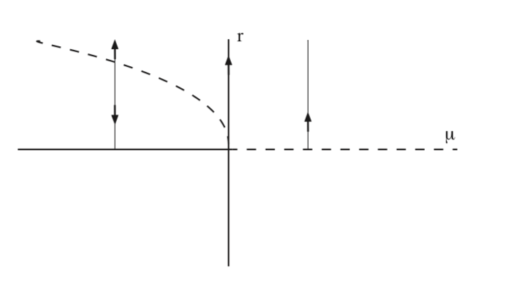
Using this information, we analyze the behavior of Equation \ref{9.12} by constructing the bifurcation diagram. There are two cases to consider: \(a > 0\) and \(a < 0\).
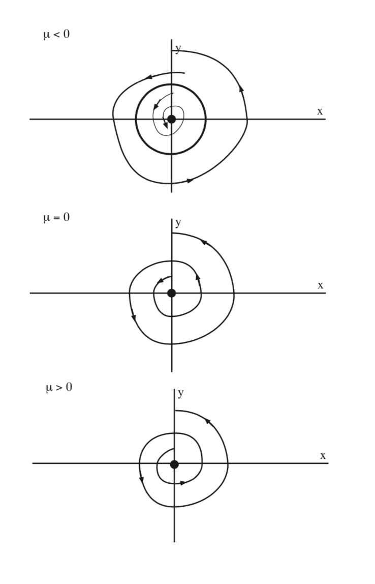
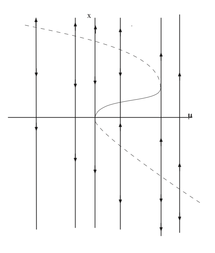
In figure 9.1 we sketch the zeros of (9.12) as a function of \(\mu\) for a > 0. We see that a periodic orbit bifurcates from the nonhyperbolic fixed point at \(\mu = 0\). The periodic orbit is unstable and exists for \(\mu < 0\). In Fig. 9.2 we illustrate the dynamics in the \(x - y\) phase plane.
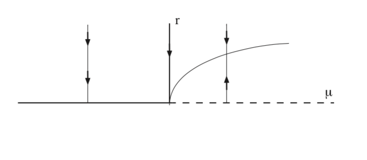
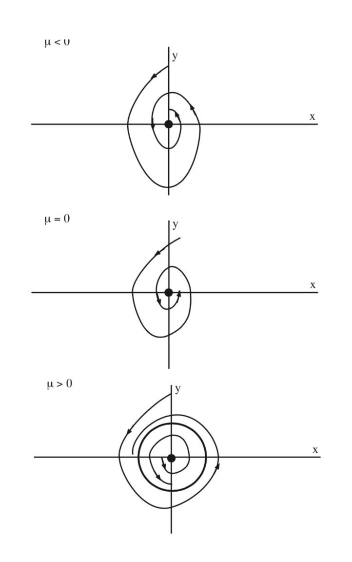
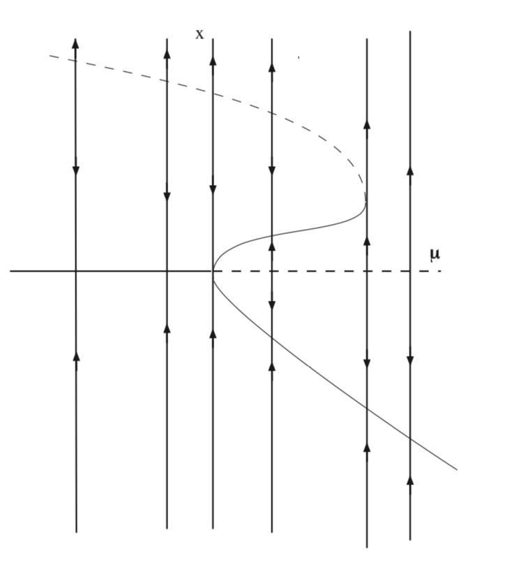
In figure 9.3 we sketch the zeros of Equation \ref{9.12} as a function of \(\mu\) for a < 0. We see that a periodic orbit bifurcates from the nonhyperbolic fixed point at \(\mu = 0\). The periodic orbit is stable in this case and exists for \(\mu > 0\). In Fig. 9.4 we illustrate the dynamics in the \(x - y\) phase plane.
In this example we have seen that a nonhyperbolic fixed point of a two dimensional autonomous vector field, where the nonhyperbolicity arises from the fact that the linearization at the fixed point has a pair of pure imaginary eigenvalues, \(\pm i\mathcal{w}\), can lead to the creation of periodic orbits as a parameter is varied. This is an example of what is generally called the Hopf bifurcation. It is the first example we have seen of the bifurcation of an equilibrium solution resulting in time-dependent solutions.
At this point it is useful to summarize the nature of the conditions resulting in a Hopf bifurcation for a two dimensional, autonomous vector field. To begin with, we need a fixed point where the Jacobian associated with the linearization about the fixed point has a pair of pure imaginary eigenvalues. This is a necessary condition for the Hopf bifurcation. Now just as for bifurcations of fixed points of one dimensional autonomous vector fields (e.g., the saddle-node, transcritical, and pitchfork bifurcations that we have studied in the previous chapter) the nature of the bifurcation for parameter values in a neighbourhood of the bifurcation parameter is determined by the form of the nonlinearity of the vector field. We developed the idea of the Hopf bifurcation in the context of Equation \ref{9.1}, and in that example the stability of the bifurcating periodic orbit was given by the sign of the coefficient a (stable for a < 0, unstable for a > 0). In the example the âA ̆ŸâA ̆Z ́stability coefficient âA ̆Z ́âA ̆Z ́was evident from the simple structure of the nonlinearity. In more complicated examples, i.e. more complicated nonlinear terms, the determination of the stability coefficient is more âA ̆ŸâA ̆Z ́algebraically intensive âA ̆Z ́âA ̆Z ́.Explicit expressions for the stability coefficient are given in many dynamical systems texts. For example, it is given in Guckenheimer and Holmes and Wiggins. The complete details of the calculation of the stability coefficient are carried out in 7. Problem 2 at the end of this chapter explores the nature of the Hopf bifurcation, e.g. the number and stability of bifurcating periodic orbits, for different forms of nonlinearity.
Next, we return to the examples of bifurcations of fixed points in one dimensional vector fields and give two examples of one dimensional vector fields where more than one of the bifurcations we discussed earlier can occur.
Example \(\PageIndex{27}\)
Consider the following one dimensional autonomous vector field depending on a parameter \(\mu\):
\[\dot{x} = \mu-\frac{x^2}{2}+\frac{x^3}{3} , x \in \mathbb{R}. \label{9.16}\]
The fixed points of this vector field are given by:
\[\mu = \frac{x^2}{2}-\frac{x^3}{3}, \label{9.17}\]
and are plotted in Fig. 9.5.
The curve plotted is where the vector field is zero. Hence, it is positive to the right of the curve and negative to the left of the curve. From this we conclude the stability of the fixed points as shown in the figure.
There are two saddle node bifurcations that occur where \(\frac{d \mu}{dx} (x) = 0\). These are located at
\[(x, \mu) = (0, 0), (1,\frac{1}{6}). \label{9.18}\]
Example \(\PageIndex{28}\)
Consider the following one dimensional autonomous vector field depending on a parameter \(\mu\):
\(\dot{x} = \mu x-\frac{x^3}{2}+\frac{x^4}{3}\),
\[= x(\mu-\frac{x^2}{2}+\frac{x^3}{3}), \label{9.19}\]
The fixed points of this vector field are given by:
\[\mu = \frac{x^2}{2}-\frac{x^3}{3}, \label{9.20}\]
and
\[x = 0, \label{9.21}\]
and are plotted in the \(\mu - x\) plane in Fig. 9.6.
In this example we see that there is a pitchfork bifurcation and a saddle-node bifurcation.