10.1: Center Manifold Theory
- Page ID
- 24193

This chapter is about center manifolds, dimensional reduction, and stability of fixed points of autonomous vector fields. We begin with a motivational example.
Example \(\PageIndex{29}\)
Consider the following linear, autonomous vector field on \(\mathbb{R}^{c} \times \mathbb{R}^s\):
\(\dot{x} = Ax\),
\[\dot{y} = By, (x, y) \in \mathbb{R} \times \mathbb{R}, \label{10.1}\]
where A is a \(c \times c\) matrix of real numbers having eigenvalues with zero real part and \(B\) is a \(s \times s\) matrix of real numbers having eigenvalues with negative real part. Suppose we are interested in stability of the nonhyperbolic fixed point \((x, y) = (0, 0)\). Then that question is determined by the nature of stability of \(x = 0\) in the lower dimensional vector field:
\[\dot{x} = Ax, x \in \mathbb{R}^c. \label{10.2}\]
This follows from the nature of the eigenvalues of \(B\), and the properties that \(x\) and \(y\) are decoupled in (10) and that it is linear. More precisely, the solution of (10) is given by:
\[\begin{pmatrix} {x(t, x_{0})}&{y(t, y_{0}) } \end{pmatrix} = \begin{pmatrix} {e^{At}x_{0}}&{e^{Bt}y_{0}} \end{pmatrix}. \label{10.3}\]
From the assumption of the real parts of the eigenvalues of B having negative real parts, it follows that:
\[\lim_{t \rightarrow \infty} e^{Bt}y_{0} = 0.\]
In fact, 0 is approached at an exponential rate in time. Therefore it follows that stability, or asymptotic stability, or instability of x = 0 for (10.2) implies stability, or asymptotic stability, or instability of (x, y) = (0, 0) for (10).
It is natural to ask if such a dimensional reduction procedure holds for nonlinear systems. This might seem unlikely since, in general, nonlinear systems are coupled and the superposition principle of linear systems does not hold. However, we will see that this is not the case.
Invariant manifolds lead to a form of decoupling that results in a dimensional reduction procedure that gives, essentially, the same result as is obtained for this motivational linear example.This is the topic of center manifold theory that we now develop.
We begin by describing the set-up. It is important to realize that when applying these results to a vector field, it must be in the following form.
\(\dot{x} = Ax+f(x, y)\),
\[\dot{y} = By + g(x, y), (x, y) \in \mathbb{R}^c \times \mathbb{R}^s, \label{10.4}\]
where the matrices A and B are have the following properties:
- \(c \times c\) matrix of real numbers having eigenvalues with zero real parts,
- \(s \times s\) matrix of real numbers having eigenvalues with negative real parts,
and \(f\) and \(g\) are nonlinear functions. That is, they are of order two or higher in x and y, which is expressed in the following properties:
\[f(0, 0) = 0, Df(0, 0) = 0\]
\[g(0, 0) = 0, Dg(0, 0) = 0, \label{10.5}\]
and they are \(C^r\), \(r\) as large as required (we will explain what this means when we explicitly use this property later on).
With this set-up (x, y) = (0, 0) is a fixed point for (10.4) and we are interested in its stability properties.
The linearization of (10.4) about the fixed point is given by:
\(\dot{x} = Ax\),
\[\dot{y} = By, (x, y) \in \mathbb{R}^{c} \times \mathbb{R}^{s}, \label{10.6}\]
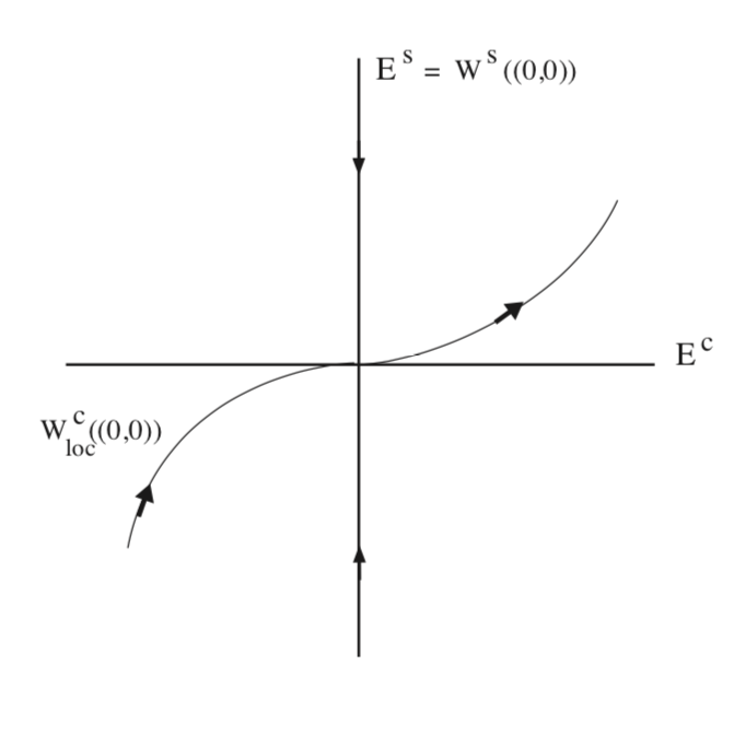
The fixed point is nonhyperbolic. It has a c dimensional invariant center subspace and a s dimensional invariant stable subspace given by:
\[E^c = {(x, y) \in R^{c} \times R^{s} | y = 0}, \label{10.7}\]
\[E^s = {(x, y) \in R^{c} \times R^{s} | x = 0}, \label{10.8}\]
respectively.
For the nonlinear system (Equation \ref{10.4}) there is a s dimensional, \(C^r\) passing through the origin and tangent to \(E^s\) at the origin. Moreover, trajectories in the local stable manifold inherit their behavior from trajectories in \(E^s\) under the linearized dynamics in the sense that they approach the origin at an exponential rate in time.
Similarly, there is a c dimensional \(C^r\) local center manifold that passes through the origin and is tangent to \(E^c\) are the origin. Hence, the center manifold has the form:
\[W^{c}(0) = {(x, y) \in \mathbb{R}^c \times \mathbb{R}^s | y = h(x), h(0) = 0, Dh(0) = 0}, \label{10.9}\]
which is valid in a neighborhood of the origin, i.e. for |x| sufficiently small.
We illustrate the geometry in Fig. 10.1.
The application of the center manifold theory for analyzing the behavior of trajectories near the origin is based on three theorems:
- existence of the center manifold and the vector field restricted to the center manifold,
- stability of the origin restricted to the center manifold and its relation to the stability of the origin in the full dimensional phase space,
- obtaining an approximation to the center manifold.
Theorem 5: Existence and Restricted Dynamics
There exists a \(C^r\) center manifold of \((x, y) = (0, 0)\) for Equation \ref{10.4}. The dynamics of Equation \ref{10.4} restricted to the center manifold is given by:
\[\dot{u} = Au+f(u, h(u)), u \in \mathbb{R}^c, \label{10.10}\]
for |u| sufficiently small.
A natural question that arises from the statement of this theorem is "why did we use the variable'‘u' when it would seem that 'x' would be the more natural variable to use in this situation"? Understanding the answer to this question will provide some insight and understanding to the nature of solutions near the origin and the geometry of the invariant manifolds near the origin. The answer is that "x and y are already used as variables for describing the coordinate axes in Equation \ref{10.4}. We do not want to confuse a point in the center manifold with a point on the coordinate axis. A point on the center manifold is denoted by (x, h(x)). The coordinate u denotes a parametric representation of points along the center manifold. Moreover, we will want to compare trajectories of Equation \ref{10.10} with trajectories in Equation \ref{10.4}. This will be confusing if x is used to denote a point on the center manifold. However, when computing the center manifold and when considering the (i.e. Equation \ref{10.10}) it is traditional to use the coordinate 'x', i.e. the coordinate describing the points in the center subspace. This does not cause ambiguities since we can name a coordinate anything we want. However, it would cause ambiguities when comparing trajectores in Equation \ref{10.4} with trajectories in Equation \ref{10.10}, as we do in the next theorem.
Theorem 6
- Suppose that the zero solution of Equation \ref{10.10} is stable (asymptotically stable) (unstable), then the zero solution of (10.4) is also stable (asymptotically stable) (unstable).
- Suppose that the zero solution of Equation \ref{10.10} is stable. Then if (x(t), y(t)) is a solution of (10.4) with (x(0), y(0)) sufficiently small, then there is a solution \(u(t)\) of Equation \ref{10.10} such that as \(t \rightarrow \infty\)
\(x(t) = u(t) + \mathcal{O}(e^{-\gamma t})\),
\[y(t) = h(u(t)) + \mathcal{O}(e^{-\gamma t}), \label{10.11}\]
where \(\gamma > 0\) is a constant.
Part i) of this theorem says that stability properties of the origin in the center manifold imply the same stability properties of the origin in the full dimensional equations. Part ii) gives much more precise results for the case that the origin is stable. It says that trajectories starting at initial conditions sufficiently close to the origin asymptotically approach a trajectory in the center manifold.
Now we would like to compute the center manifold so that we can use these theorems in specific examples. In general, it is not possible to compute the center manifold. However, it is possible to approximate it to "sufficiently high accuracy" so that we can verify the stability results of Theorem 6 can be confirmed. We will show how this can be done. The idea is to derive an equation that the center manifold must satisfy, and then develop an approximate solution to that equation.
We develop this approach step-by-step.
The center manifold is realized as the graph of a function,
\[y=h(x), x \in \mathbb{R}^c, y \in \mathbb{R}^s, \label{10.12}\]
i.e. any point \((x_{c}, y_{c})\), sufficiently close to the origin, that is in the center manifold satisfies \(y_{c} = h(x-{c})\). In addition, the center manifold passes through the origin (h(0) = 0) and is tangent to the center sub- space at the origin (\(Dh(0) = 0\)).
Invariance of the center manifold implies that the graph of the function \(h(x)\) must also be invariant with respect to the dynamics generated by Equation \ref{10.4}. Differentiating Equation \ref{10.12} with respect to time shows that \((\dot{x}, \dot{y})\) at any point on the center manifold satisfies
\[\dot{y} = Dh(x)\dot{x}. \label{10.13}\]
This is just the analytical manifestation of the fact that invariance of a surface with respect to a vector field implies that the vector field must be tangent to the surface.
We will now use these properties to derive an equation that must be satisfied by the local center manifold.
The starting point is to recall that any point on the local center manifold obeys the dynamics generated by . Substituting y = h(x) into gives:
\[\dot{x} = Ax + f (x, h(x)), \label{10.14}\]
\[\dot{y} = Bh(x) + g(x, h(x)), (x, y) \in \mathbb{R}^c \times \mathbb{R}^s. \label{10.15}\]
Substituting and into the invariance condition \(\dot{y} = Dh(x)\dot{x}\) gives:
\[Bh(x) + g(x, h(x)) = Dh(x) (Ax + f (x, h(x))) , \label{10.16}\]
or
\[Dh(x)(Ax+f(x, h(x)))-Bh(x)-g(x, h(x)) \equiv \mathcal{N}(h(x) = 0. \label{10.17}\]
This is an equation for \(h(x)\). By construction, the solution implies invariance of the graph of \(h(x)\), and we seek a solution satisfying the additional conditions \(h(0) = 0\) and \(Dh(0) = 0\). The basic result on approximation of the center manifold is given by the following theorem.
Theorem 7: Approximation
Let \(\phi : \mathbb{R}^c \rightarrow \mathbb{R}^s\) be a \(C^1\) mapping with
\(\phi (0) = 0, D_{\phi}(0) = 0\),
such that
\(\mathcal{N}(\phi (x)) = \mathcal{O}(|x|^{q})\) as \(x \rightarrow 0\),
for some \(q > 1\). Then
\(|h(x)-\phi (x)| = \mathcal{O}(|x|^{q})\) as \(x \rightarrow 0\).
The theorem states that if we can find an approximate solution of Equation \ref{10.17} to a specified degree of accuracy, then that approximate solution is actually an approximation to the local center manifold, to the same degree of accuracy.
We now consider some examples showing how these results are applied.
Example \(\PageIndex{30}\)
We consider the following autonomous vector field on the plane:
\(\dot{x} = x^{2}y-x^5\),
\[\dot{y} = -y+x^2, (x, y) \in \mathbb{R}^2, \label{10.18}\].
or, in matrix form:
\[\begin{pmatrix} {\dot{x}}\\ {\dot{y}} \end{pmatrix} = \begin{pmatrix} {0}&{0}\\ {0}&{-1} \end{pmatrix} \begin{pmatrix} {x}\\ {y} \end{pmatrix} + \begin{pmatrix} {x^{2}y-x^5}\\ {x^2} \end{pmatrix}, \label{10.19}\]
We are interested in determining the natural of the stability of (x, y) = (0, 0). The Jacobian associated with the linearization about this fixed point is:
\(\begin{pmatrix} {0}&{0}\\ {0}&{-1} \end{pmatrix}\),
which is nonhyperbolic, and therefore the linearization does not suffice to determine stability.
The vector field is in the form of Equation \ref{10.4}
\(\dot{x} = Ax+f(x, y)\),
\[\dot{y} = By+g(x, y), (x, y) \in \mathbb{R} \times \mathbb{R}, \label{10.20}\]
where
\[A = 0, B = 1, f(x, y)=x^{2}y-x^5, g(x, y) = x^2. \label{10.21}\]
We assume a center manifold of the form:
\[y = h(x) = ax^2 + bx^3 + \mathcal{O}(x^4), \label{10.22}\]
which satisfies h(0) = 0 ("passes through the origin") and Dh(0) = 0 (tangent to \(E^{c}\) at the origin). A center manifold of this type will require the vector field to be at least \(C^3\) (hence, the meaning of the phrase \(C^r\), r as large as necessary).
Substituting this expression into the equation for the center manifold (10.17) (using (10.21)) gives:
\[(2ax+3b^{2}+\mathcal{O}(x^3))(ax^4+bx^5+\mathcal{O}(x^6)-x^5)+ax^2+bx^3+\mathcal{O}(x^4)-x^2 = 0. \label{10.23}\]
In order for this equation to be satisfied the coefficients on each power of x must be zero. Through third order this gives:
\(x^2 : a - 1 = 0 \Rightarrow a = 1\),
\[x^3 : b = 0. \label{10.24}\]
Substituting these values into (10.22) gives the following expression for the center manifold through third order:
\[y = x^2 + \mathcal{O}(x^4). \label{10.25}\]
Therefore the vector field restricted to the center manifold is given by:
\[\dot{x} = x^4 + \mathcal{O}(x^5). \label{10.26}\]
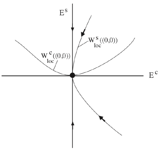
Hence, for x sufficiently small, \(\dot{x}\) is positive for \(x \ne 0\), and therefore the origin is unstable. We illustrate the flow near the origin in Fig. 10.2.
Example \(\PageIndex{31}\)
We consider the following autonomous vector field on the plane:
\(\dot{x} = xy\),
\[\dot{y} = y+x^3, (x, y) \in \mathbb{R}^2, \label{10.27}\]
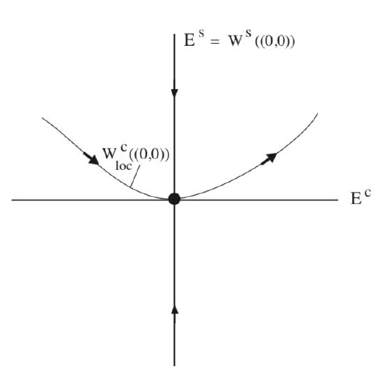
Therefore the vector field restricted to the center manifold is given by:
\[\dot{x} = x^4 + \mathcal{O}(x^5). \label{10.35}\]
Since \(\dot{x}\) is positive for x sufficiently small. the origin is unstable. We illustrate the flow near the origin in Fig. 10.3.