1.0: Introduction

Preface

These lecture notes are intented as a straightforward introduction to partial differential equations which can serve as a textbook for undergraduate and beginning graduate students.

For additional reading we recommend following books: W. I. Smirnov [21], I. G. Petrowski [17], P. R. Garabedian [8], W. A. Strauss [23], F. John [10], L. C. Evans [5] and R. Courant and D. Hilbert[4] and D. Gilbarg and N. S. Trudinger [9]. Some material of these lecture notes was taken from some of these books.

Introduction

Ordinary and partial differential equations occur in many applications. An ordinary differential equation is a special case of a partial differential equation but the behavior of solutions is quite different in general caused by the fact that the functions for which we are looking at are functions of more than one independent variable.

Equation

$$F(x,y(x),y'(x),\ldots,y^{(n)})=0\]

is an ordinary differential equation of n-th order for the unknown function \(y(x)\), where \(F\) is given.

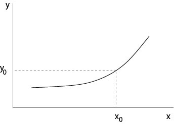
An important problem for ordinary differential equations is the initial value problem

\begin{eqnarray*}
y'(x)&=&f(x,y(x))\\
y(x_0)&=&y_0\ ,
\end{eqnarray*}

where \(f\) is a given real function of two variables \(x\),\(y\) and \(x_0,\), \( y_0\) are given real numbers.

Picard-Lindelöf Theorem. Suppose
(i) \(f(x,y)\) is continuous in a rectangle

$$Q=\{(x,y)\in{{\mathbb R}^2}:\ |x-x_0|<a,\ |y-y_0|<b\}.$$

(ii) There is a constant \(K\) such that \(|f(x,y)|\le K\) for all \((x,y) \in Q\).
(ii) Lipschitz condition: There is a constant \(L\) such that

$$|f(x,y_2)-f(x,y_1)|\le L|y_2-y_1|$$

for all \((x,y_1), (x,y_2)\).

Figure 1.0.1: Initial value problem

Then there exists a unique solution \(y\in C^1(x_0-\alpha,x_0+\alpha)\) of the above initial value problem, where \(\alpha=\min (b/K,a)\).

The linear ordinary differential equation

$$y^{(n)}+a_{n-1}(x)y^{(n-1)}+\ldots a_1(x)y'+a_0(x)y=0,\]

where \(a_j\) are continuous functions, has exactly \(n\) linearly independent solutions. In contrast to this property the partial differential \(u_{xx}+u_{yy}=0\) in \({\mathbb R}^2\) has infinitely many linearly independent solutions in the linear space \(C^2(\mathbb{R})^2\).

The ordinary differential equation of second order

$$y''(x)=f(x,y(x),y'(x))\]

has in general a family of solutions with two free parameters. Thus, it is naturally to consider the associated initial value problem

\begin{eqnarray*}
y''(x)&=&f(x,y(x),y'(x))\\
y(x_0)&=&y_0,\ y'(x_0)=y_1,
\end{eqnarray*}
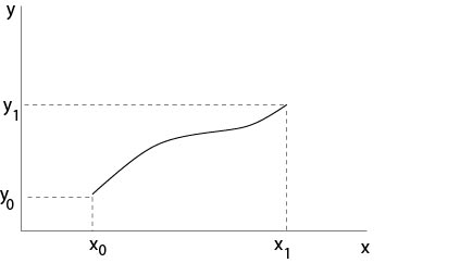
where \(y_0\) and \(y_1\) are given, or to consider the boundary value problem
\begin{eqnarray*}
y''(x)&=&f(x,y(x),y'(x))\\
y(x_0)&=&y_0,\ y(x_1)=y_1.
\end{eqnarray*}

Figure 1.0.2: Boundary value problem

Initial and boundary value problems play an important role also in the theory of partial differential equations. A partial differential equation for the unknown function \(u(x,y)\) is for example

$$F(x,y,u,u_x,u_y,u_{xx},u_{xy},u_{yy})=0,\]

where the function \(F\) is given. This equation is of second order.

An equation is said to be of n-th order if the highest derivative which occurs is of order \(n\).

An equation is said to be linear if the unknown function and its derivatives are linear in \(F\). For example,

$$a(x,y)u_x+b(x,y)u_y+c(x,y)u=f(x,y),\]

where the functions \(a\),\(b\),\(c\) and \(f\) are given, is a linear equation of first order.

An equation is said to be quasilinear if it is linear in the highest derivatives. For example,

$$a(x,y,u,u_x,u_y)u_{xx}+b(x,y,u,u_x,u_y)u_{xy}+c(x,y,u,u_x,u_y)u_{yy}=0\]

is a quasilinear equation of second order.

Contributors and Attributions

• Prof. Dr. Erich Miersemann (Universität Leipzig)

• Integrated by Justin Marshall.