1.1: Examples

Example 1.1.1:

$u_y=0$, where $u=u(x,y)$. All functions $u=w(x)$ are solutions.

Example 1.1.2:

$u_x=u_y$, where $u=u(x,y)$. A change of coordinates transforms this equation into an equation of the first example. Set $\xi=x+y,\ \eta=x-y$, then
$$u(x,y)=u\left(\frac{\xi+\eta}{2},\frac{\xi-\eta}{2}\right)=:v(\xi,\eta).$$
Assume $u\in C^1$, then
$$v_\eta=\frac{1}{2}(u_x-u_y).$$
If $u_x=u_y$, then $v_\eta=0$ and vice versa, thus $v=w(\xi)$ are solutions for arbitrary $C^1$-functions $w(\xi)$. Consequently, we have a large class of solutions of the original partial differential equation: $u=w(x+y)$ with an arbitrary $C^1$-function $w$.

Example 1.1.3:

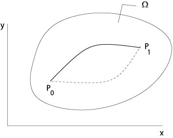
A necessary and sufficient condition such that for given $C^1$-functions $M,\ N$ the integral
$$\int_{P_0}^{P_1}\ M(x,y)dx+N(x,y)dy$$
is independent of the curve which connects the points $P_0$ with $P_1$ in a simply connected domain $\Omega\subset\mathbb{R}^2$ is that the partial differential equation (condition of integrability)
$$M_y=N_x$$
in $\Omega$.

Figure 1.1.1: Independence of the path

This is one equation for two functions. A large class of solutions is given by $M=\Phi_x,\ N=\Phi_y$, where $\Phi(x,y)$ is an arbitrary $C^2$-function. It follows from Gauss theorem that these are all $C^1$-solutions of the above differential equation.

Example 1.1.4: Method of an integrating multiplier for an ordinary

differential

equation

Consider the ordinary differential equation
$$M(x,y)dx+N(x,y)dy=0$$
for given $C^1$-functions $M,\ N$. Then we seek a $C^1$-function $\mu(x,y)$ such that $\mu Mdx+\mu Ndy$ is a total differential, i. e., that $(\mu M)_y=(\mu N)_x$ is satisfied. This is a linear partial differential equation of first order for $\mu$:
$$
M\mu_y-N\mu_x=\mu (N_x-M_y).
\]

Example 1.1.5:

Two $C^1$-functions $u(x,y)$ and $v(x,y)$ are said to be functionally dependent if
$$\det\left(\begin{array}{cc}u_x&u_y\\v_x&v_y\end{array}\right)=0,$$
which is a linear partial differential equation of first order for $u$ if $v$ is a given $C^1$-function. A large class of solutions is given by
$$u=H(v(x,y)),$$
where $H$ is an arbitrary $C^1$-function.

Example 1.1.6: Cauchy-Riemann equations

Set $f(z)=u(x,y)+iv(x,y)$, where $z=x+iy$ and $u,\ v$ are given $C^1(\Omega)$-functions. Here $\Omega$ is a domain in $\mathbb{R}^2$. If the function $f(z)$ is differentiable with respect to the complex variable $z$ then $u,\ v$ satisfy the Cauchy-Riemann equations
$$u_x=v_y,\ \ u_y=-v_x.$$
It is known from the theory of functions of one complex variable that the real part $u$ and the imaginary part $v$ of a differentiable function $f(z)$ are solutions of the Laplace equation
$$\triangle u=0,\ \ \triangle v=0,$$
where $\triangle u= u_{xx}+u_{yy}$.

Example 1.1.7: Newton Potential

The Newton potential
$$u=\frac{1}{\sqrt{x^2+y^2+z^2}}$$
is a solution of the Laplace equation in $\mathbb{R}^3\setminus{(0,0,0)}$, that is, of
$$
u_{xx}+u_{yy}+u_{zz}=0.
\]

Example 1.1.8: Heat equation

Let $u(x,t)$ be the temperature of a point $x\in\Omega$ at time $t$, where $\Omega\subset\mathbb{R}^3$ is a domain. Then $u(x,t)$ satisfies in $\Omega\times[0,\infty)$ the heat equation
$$u_t=k\triangle u,$$
where $\triangle u= u_{x_1x_1}+u_{x_2x_2}+u_{x_3x_3}$ and $k$ is a positive constant. The condition
$$u(x,0)=u_0(x),\ \ x\in \Omega,$$
where $u_0(x)$ is given, is an initial condition associated to the above heat equation. The condition
$$u(x,t)=h(x,t),\ \ x\in \partial\Omega,\ t\ge0,$$
where $h(x,t)$ is given, is a boundary condition for the heat equation.

If $h(x,t)=g(x)$, that is, $h$ is independent of $t$, then one expects that the solution $u(x,t)$ tends to a function $v(x)$ if $t\to\infty$. Moreover, it turns out that $v$ is the solution of the boundary value problem for the Laplace equation
$$\begin{eqnarray*} \triangle v&=&0\ \ \mbox{in}\ \Omega\\ v&=&g(x)\ \ \mbox{on}\ \partial\Omega. \end{eqnarray*}$$

Example 1.1.9: Wave equation

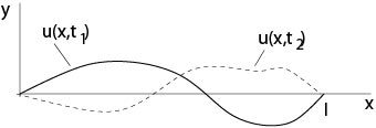
Figure 1.1.2: Oscillating string

The wave equation
$$u_{tt}=c^2\triangle u,$$
where $u=u(x,t)$, $c$ is a positive constant, describes oscillations of membranes or of three dimensional domains, for example. In the one-dimensional case
$$u_{tt}=c^2 u_{xx}$$
describes oscillations of a string.

Associated initial conditions are
$$u(x,0)=u_0(x),\ \ u_t(x,0)=u_1(x),$$
where $u_0,\ u_1$ are given functions. Thus the initial position and the initial velocity are prescribed.

If the string is finite one describes additionally boundary conditions, for example
$$
u(0,t)=0,\ \ u(l,t)=0\ \ \mbox{for all}\ t\ge 0.
\]

Contributors and Attributions

• Prof. Dr. Erich Miersemann (Universität Leipzig)

• Integrated by Justin Marshall.