2.5: Hamilton-Jacobi Theory

The nonlinear equation (2.4.1) of previous section in one more dimension is

$$
F(x_1,\ldots,x_n,x_{n+1},z,p_1,\ldots,p_n,p_{n+1})=0.
\]

The content of the Hamilton¹-Jacobi² theory is the theory of the special case

\begin{equation}
\label{nonlinearham}
F\equiv p_{n+1}+H(x_1,\ldots,x_n,x_{n+1},p_1,\ldots,p_n)=0,
\end{equation}

i. e., the equation is linear in \(p_{n+1}\) and does not depend on \(z\) explicitly.

Remark. Formally, one can write equation (2.4.1)

$$F(x_1,\ldots,x_n,u,u_{x_1},\ldots,u_{x_n})=0\]

as an equation of type (\ref{nonlinearham}). Set \(x_{n+1}=u\) and seek \(u\) implicitly from

$$\phi(x_1,\ldots,x_n,x_{n+1})=const.,\]

where \(\phi\) is a function which is defined by a differential equation.

Assume \(\phi_{x_{n+1}}\not=0\), then

\begin{eqnarray*}
0&=&F(x_1,\ldots,x_n,u,u_{x_1},\ldots,u_{x_n})\\
&=&F(x_1,\ldots,x_n,x_{n+1},-\frac{\phi_{x_1}}{\phi_{x_{n+1}}},\ldots,-\frac{\phi_{x_n}}{\phi_{x_{n+1}}})\\
&=&:G(x_1,\ldots,x_{n+1},\phi_1,\ldots,\phi_{x_{n+1}}).
\end{eqnarray*}

Suppose that \(G_{\phi_{x_{n+1}}}\not=0\), then

$$\phi_{x_{n+1}}=H(x_1,\ldots,x_n,x_{n+1},\phi_{x_1},\ldots,\phi_{x_{n+1}}).\]

The associated characteristic equations to (\ref{nonlinearham}) are

\begin{eqnarray*}
x_{n+1}'(\tau)&=&F_{p_{n+1}}=1\\
x_k'(\tau)&=&F_{p_k}=H_{p_k},\qquad k=1,\ldots,n\\
z'(\tau)&=&\sum_{l=1}^{n+1} p_lF_{p_l}=\sum_{l=1}^np_lH_{p_l}+p_{n+1}\\
&=&\sum_{l=1}^np_lH_{p_l}-H\\
p'_{n+1}(\tau)&=&-F_{x_{n+1}}-F_zp_{n+1}\\
&=&-F_{x_{n+1}}\\
p_k'(\tau)&=&-F_{x_k}-F_zp_k\\
&=&-F_{x_k},\qquad k=1,\ldots,n.
\end{eqnarray*}

Set \(t:=x_{n+1}\), then we can write partial differential equation (\ref{nonlinearham}) as

\begin{equation}
\label{hamjac}
u_t+H(x,t,\nabla_xu)=0
\end{equation}
and \(2n\) of the characteristic equations are
\begin{eqnarray}
\label{charhj1}
x'(t)&=&\nabla_pH(x,t,p)\\
\label{charhj2}
p'(t)&=&-\nabla_xH(x,t,p).
\end{eqnarray}
Here is

$$x=(x_1,\ldots,x_n),\ p=(p_1,\ldots,p_n).\]

Let \(x(t),\ p(t)\) be a solution of (\ref{charhj1}) and (\ref{charhj2}), then it follows \(p_{n+1}'(t)\) and \(z'(t)\) from the characteristic equations

\begin{eqnarray*}
p'_{n+1}(t)&=&-H_t\\
z'(t)&=&p\cdot\nabla_pH-H.
\end{eqnarray*}

Definition. The function \(H(x,t,p)\) is called Hamilton function, equation (\ref{nonlinearham}) Hamilton-Jacobi equation and the system (\ref{charhj1}), (\ref{charhj2}) canonical system to H.

There is an interesting interplay between the Hamilton-Jacobi equation and the canonical system. According to the previous theory we can construct a solution of the Hamilton-Jacobi equation by using solutions of the canonical system. On the other hand, one obtains from solutions of the Hamilton-Jacobi equation also solutions of the canonical system of ordinary differential equations.

Definition.
A solution \(\phi(a;x,t)\) of the Hamilton-Jacobi equation, where \(a=(a_1,\ldots,a_n)\) is an \(n\)-tuple of real parameters, is called a complete integral of the Hamilton-Jacobi equation if
$$
\det (\phi_{x_ia_l})_{i,l=1}^n\not=0.
\]

Remark. If \(u\) is a solution of the Hamilton-Jacobi equation, then also \(u+const.\)

Theorem 2.4 (Jacobi). Assume

$$u=\phi(a;x,t)+c,\ c=const.,\ \phi\in C^2\ \mbox{in its arguments},$$

is a complete integral. Then one obtains by solving of

$$b_i=\phi_{a_i}(a;x,t)$$

with respect to \(x_l=x_l(a,b,t)\), where \(b_i\ i=1,\ldots,n\) are given real constants, and then by setting

$$p_k=\phi_{x_k}(a;x(a,b;t),t)$$

a 2n-parameter family of solutions of the canonical system.

Proof. Let

$$x_l(a,b;t),\ l=1,\ldots,n,\]

be the solution of the above system. The solution exists since \(\phi\) is a complete integral by assumption. Set

$$p_k(a,b;t)=\phi_{x_k}(a;x(a,b;t),t),\ k=1,\ldots,n.\]

We will show that \(x\) and \(p\) solves the canonical system. Differentiating \(\phi_{a_i}=b_i\) with respect to \(t\) and the Hamilton-Jacobi equation \(\phi_t+H(x,t,\nabla_x\phi)=0\) with respect to \(a_i\), we obtain for \(i=1,\ldots,n\)

\begin{eqnarray*}
\phi_{ta_i}+\sum_{k=1}^n\phi_{x_ka_i}\frac{\partial x_k}{\partial t}&=&0\\
\phi_{ta_i}+\sum_{k=1}^n\phi_{x_ka_i}H{p_k}&=&0.
\end{eqnarray*}
Since \(\phi\) is a complete integral it follows for \(k=1,\ldots,n\)

$$\frac{\partial x_k}{\partial t}=H_{p_k}.\]

Along a trajectory, i. e., where \(a,\ b\) are fixed, it is \(\frac{\partial x_k}{\partial t}=x_k'(t)\). Thus

$$x_k'(t)=H_{p_k}.\]

Now we differentiate \(p_i(a,b;t)\) with respect to \(t\) and \(\phi_t+H(x,t,\nabla_x\phi)=0\) with respect to \(x_i\), and obtain

\begin{eqnarray*}
p_i'(t)&=&\phi_{x_it}+\sum_{k=1}^n\phi_{x_ix_k}x_k'(t)\\
0&=&\phi_{x_it}+\sum_{k=1}^n\phi_{x_ix_k}H_{p_k}+H_{x_i}\\
0&=&\phi_{x_it}+\sum_{k=1}^n\phi_{x_ix_k}x_k'(t)+H_{x_i}
\end{eqnarray*}

It follows finally that \(p_i'(t)=-H_{x_i}\).

\(\Box\)

Example 2.5.1: Kepler problem

The motion of a mass point in a central field takes place in a plane, say the \((x,y)\)-plane, see Figure 2.5.1, and satisfies the system of ordinary differential equations of second order

$$x''(t)=U_x,\ y''(t)=U_y,\]

where

$$U(x,y)=\frac{k^2}{\sqrt{x^2+y^2}}.\]

Here we assume that \(k^2\) is a positive constant and that the mass point is attracted of the origin. In the case that it is pushed one has to replace \(U\) by \(-U\). See Landau and Lifschitz [12], Vol 1, for instance, concerning the related physics.

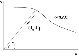
Figure 2.5.1: Motion in a central field

Set

$$p=x',\ q=y'\]

and

$$H=\frac{1}{2}(p^2+q^2)-U(x,y),\]

then

\begin{eqnarray*}
x'(t)&=&H_p,\ y'(t)=H_q\\
p'(t)&=&-H_x,\ q'(t)=-H_y.
\end{eqnarray*}
The associated Hamilton-Jacobi equation is
\begin{equation*}
\phi_t+\frac{1}{2}(\phi_x^2+\phi_y^2)=\frac{k^2}{\sqrt{x^2+y^2}}.
\end{equation*}
which is in polar coordinates \((r,\theta)\)
\begin{equation}
\label{keplerhj}
\phi_t+\frac{1}{2}(\phi_r^2+\frac{1}{r^2}\phi_\theta^2)=\frac{k^2}{r}.
\end{equation}
Now we will seek a complete integral of (\ref{keplerhj}) by making the ansatz
\begin{equation}
\label{ansatzhj}
\phi_t=-\alpha=const.\ \ \phi_\theta=-\beta=const.
\end{equation}
and obtain from (\ref{keplerhj}) that
$$
\phi=\pm\int_{r_0}^r\ \sqrt{2\alpha+\frac{2k^2}{\rho}-\frac{\beta^2}{\rho^2}}\ d\rho+c(t,\theta).
$$
From ansatz (\ref{ansatzhj}) it follows
$$
c(t,\theta)=-\alpha t-\beta\theta.
$$
Therefore we have a two parameter family of solutions
$$
\phi=\phi(\alpha,\beta;\theta,r,t)
$$
of the Hamilton-Jacobi equation. This solution is a complete integral, see an exercise.
According to the theorem of Jacobi set
$$
\phi_\alpha=-t_0,\ \ \phi_\beta=-\theta_0.
$$
Then
$$
t-t_0=-\int_{r_0}^r\ \frac{d\rho}{\sqrt{2\alpha+\frac{2k^2}{\rho}-\frac{\beta^2}{\rho^2}}}.
$$
The inverse function \(r=r(t)\), \(r(0)=r_0\), is the \(r\)-coordinate depending on time \(t\), and
$$
\theta-\theta_0=\beta\int_{r_0}^r\ \frac{d\rho}{\rho^2\sqrt{2\alpha+\frac{2k^2}{\rho}-\frac{\beta^2}{\rho^2}}}.
$$
Substitution \(\tau=\rho^{-1}\) yields
\begin{eqnarray*}
\theta-\theta_0&=&-\beta\int_{1/r_0}^{1/r}\ \frac{d\tau}{\sqrt{2\alpha+2k^2\tau-\beta^2\tau^2}}\\
&=&-\arcsin\Bigg(\frac{\frac{\beta^2}{k^2}\frac{1}{r}-1}{\sqrt{1+\frac{2\alpha\beta^2}{k^4}}}\Bigg)
+
\arcsin\Bigg(\frac{\frac{\beta^2}{k^2}\frac{1}{r_0}-1}{\sqrt{1+\frac{2\alpha\beta^2}{k^4}}}\Bigg).
\end{eqnarray*}
Set
$$
\theta_1=\theta_0+\arcsin\Bigg(\frac{\frac{\beta^2}{k^2}\frac{1}{r_0}-1}{\sqrt{1+\frac{2\alpha\beta^2}{k^4}}}\Bigg)
$$
and
$$
p=\frac{\beta^2}{k^2},\ \ \epsilon^2=\sqrt{1+\frac{2\alpha\beta^2}{k^4}},
$$
then
$$
\theta-\theta_1=-\arcsin\left(\frac{\frac{p}{r}-1}{\epsilon^2}\right).
$$
It follows
$$
r=r(\theta)=\frac{p}{1-\epsilon^2\sin(\theta-\theta_1)},
$$
which is the polar equation of conic sections. It defines an ellipse if \(0\le\epsilon<1\), a parabola if \(\epsilon=1\) and a hyperbola if \(\epsilon>1\), see Figure 2.5.2 for the case of an ellipse, where the origin of the coordinate system is one of the focal points of the ellipse.

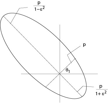
Figure 2.5.2: The case of an ellipse

For another application of the Jacobi theorem see Courant and Hilbert [4], Vol. 2, pp. 94, where geodesics on an ellipsoid are studied.

¹Hamilton, William Rowan, 1805--1865

² Jacobi, Carl Gustav, 1805--1851

Contributors and Attributions

• Prof. Dr. Erich Miersemann (Universität Leipzig)

• Integrated by Justin Marshall.