3.1: Linear Equations of Second Order

The general nonlinear partial differential equation of second order is

$$
F(x,u,Du,D^2u)=0,
$$
where \(n\), \(u:\ \Omega\subset\mathbb{R}\mapsto\mathbb{R}^1\), \(Du\equiv\nabla u\) and \(u\) stands for all second derivatives. The function \(F\) is given and sufficiently regular with respect to its \(2n+1+n^2\) arguments.

In this section we consider the case
\begin{equation}
\label{linsecond}
\sum_{i,k=1}^na^{ik}(x)u_{x_ix_k}+f(x,u,\nabla u)=0.
\end{equation}
The equation is linear if
$$
f=\sum_{i=1}^nb^i(x)u_{x_i}+c(x)u+d(x).
$$
Concerning the classification the main part
$$
\sum_{i,k=1}^n a^{ik}(x)u_{x_ix_k}
$$
plays the essential role. Suppose \(u\in C^2\), then we can assume, without restriction of generality, that \(a^{ik}=a^{ki}\), since
$$
\sum_{i,k=1}^n a^{ik}u_{x_ix_k}=\sum_{i,k=1}^n (a^{ik})^\star u_{x_ix_k},
$$
where
$$
(a^{ik})^\star=\frac{1}{2}(a^{ik}+a^{ki}).
$$
Consider a hypersurface \(\mathcal{S}\) in \(n\) defined implicitly by \(\chi(x)=0\), \(\nabla\chi\not=0\), see Figure 3.1.1

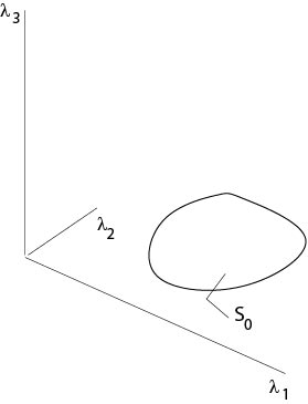
Figure 3.1.1: Initial Manifold \(\mathcal{S}\)

Assume \(u\) and \(\nabla u\) are given on \(\mathcal{S}\).

Problem: Can we calculate all other derivatives of \(u\) on \(\mathcal{S}\) by using differential equation (\ref{linsecond}\) and the given data?

We will find an answer if we map \(\mathcal{S}\) onto a hyperplane \(\mathcal{S}_0\) by a mapping
\begin{eqnarray*}
\lambda_n&=&\chi(x_1,\ldots,x_n)\\
\lambda_i&=&\lambda_i(x_1,\ldots,x_n),\ i=1,\ldots,n-1,
\end{eqnarray*}
for functions \(\lambda_i\) such that
$$
\det\frac{\partial(\lambda_1,\ldots,\lambda_n)}{\partial(x_1,\ldots,x_n)}\not=0
$$
in \(n\). It is assumed that \(i\) and \(i\) are sufficiently regular. Such a mapping \(\lambda=\lambda(x)\) exists, see an exercise.

The above transform maps \(\mathcal{S}\) onto a subset of the hyperplane defined by \(\lambda_n=0\), see Figure 3.1.2.

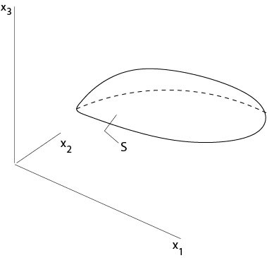
Figure 3.1.2: Transformed flat manifold \(\mathcal{S}\)

We will write the differential equation in these new coordinates. Here we use Einstein's convention, that is, we add terms with repeating indices. Since
$$
u(x)=u(x(\lambda))=:v(\lambda)=v(\lambda(x)),
$$
where \(x=(x_1,\ldots,x_n)\) and \(\lambda=(\lambda_1,\ldots,\lambda_n)\), we get
\begin{eqnarray}
\label{known}
u_{x_j}&=&v_{\lambda_i}\frac{\partial\lambda_i}{\partial x_j},\\
u_{x_jx_k}&=&v_{\lambda_i\lambda_l}\frac{\partial\lambda_i}{\partial x_j}\frac{\partial\lambda_l}{\partial x_k}+v_{\lambda_i}\frac{\partial^2\lambda_i}{\partial x_j\partial x_k}.\nonumber
\end{eqnarray}
Then the differential equation (\ref{linsecond}) in the new coordinates is given by
$$
a^{jk}(x)\frac{\partial\lambda_i}{\partial x_j}\frac{\partial\lambda_l}{\partial x_k}v_{\lambda_i\lambda_l}+\mbox{terms known on}\ \mathcal{S}_0=0.
$$
Since \(v_{\lambda_k}(\lambda_1,\ldots,\lambda_{n-1},0)\), \(n\), are known, see (\ref{known}), it follows that \(v_{\lambda_k\lambda_l}\), \(l=1,\ldots,n-1\), are known on \(\mathcal{S}_0\). Thus we know all second derivatives \(v_{\lambda_i\lambda_j}\) on \(\mathcal{S}_0\) with the only exception of \(v_{\lambda_n\lambda_n}\).

We recall that, provided \(v\) is sufficiently regular,
$$
v_{\lambda_k\lambda_l}(\lambda_1,\ldots,\lambda_{n-1},0)
$$
is the limit of
$$
\frac{v_{\lambda_k}(\lambda_1,\ldots,\lambda_l+h,\lambda_{l+1},\ldots,\lambda_{n-1},0)-
v_{\lambda_k}(\lambda_1,\ldots,\lambda_l,\lambda_{l+1},\ldots,\lambda_{n-1},0)}{h}
$$
as \(h\to0\).

Then the differential equation can be written as
$$
\sum_{j,k=1}^na^{jk}(x)\frac{\partial\lambda_n}{\partial x_j}\frac{\partial\lambda_n}{\partial x_k}v_{\lambda_n\lambda_n}=\mbox{terms known on}\ \mathcal{S}_0.
$$
It follows that we can calculate \(v_{\lambda_n\lambda_n}\) if
\begin{equation}
\label{nonchar}
\sum_{i,j=1}^na^{ij}(x)\chi_{x_i}\chi_{x_j}\not=0
\end{equation}

on \(\mathcal{S}\). This is a condition for the given equation and for the given surface \(\mathcal{S}\).

Definition. The differential equation
$$
\sum_{i,j=1}^na^{ij}(x)\chi_{x_i}\chi_{x_j}=0
$$
is called it characteristic differential equation associated to the given differential equation (\ref{linsecond}).

If \(\chi\), \(\nabla \chi\not=0\), is a solution of the characteristic differential equation, then the surface defined by \(\chi=0\) is called characteristic surface.

Remark. The condition (\ref{nonchar}) is satisfied for each \(\chi\) with \(\nabla\chi\not=0\) if the quadratic matrix \((a^{ij}(x))\) is positive or negative definite for each \(x\in\Omega\), which is equivalent to the property that all eigenvalues are different from zero and have the same sign. This follows since there is a \(\lambda(x)>0\) such that, in the case that the matrix \((a^{ij})\) is poitive definite,
$$
\sum_{i,j=1}^na^{ij}(x)\zeta_i\zeta_j\ge\lambda(x)|\zeta|^2
$$
for all \(\zeta\in\mathbb{R}\). Here and in the following we assume that the matrix \((a^{ij})\) is real and symmetric.

The characterization of differential equation (\ref{linsecond}) follows from the signs of the eigenvalues of \((a^{ij}(x))\).

Definition. The differential equation (\ref{linsecond}) is said to be of type \((\alpha,\beta,\gamma)\) at \(x\in\Omega\) if \(\alpha\) eigenvalues of \((a^{ij})(x)\) are positive, \(\beta\) eigenvalues are negative and \(\gamma\) eigenvalues are zero (\(\alpha+\beta+\gamma=n\)).
In particular, the equation is called

elliptic if it is of type \((n,0,0)\) or of type \((0,n,0)\), that is, all eigenvalues are different from zero and have the same sign,\\
parabolic if it is of type \((n-1,0,1)\) or of type \((0,n-1,1)\), that is, one eigenvalue is zero and all the others are different from zero and have the same sign,
hyperbolic if it is of type \((n-1,1,0)\) or of type \((1,n-1,0)\), that is, all eigenvalues are different from zero and one eigenvalue has another sign than all the others.

Remarks:

1. According to this definition there are other types aside from elliptic, parabolic or hyperbolic equations.

2. The classification depends in general on \(x\in\Omega\). An example is the Tricomi equation, which appears in the theory of transsonic flows,
$$
yu_{xx}+u_{yy}=0.
$$
This equation is elliptic if \(y>0\), parabolic if \(y=0\) and hyperbolic for \(y<0\).

Examples:

Example 3.1.1:

The Laplace equation in \(\mathbb{R}^3\) is \(\triangle u=0\), where
$$
\triangle u:=u_{xx}+u_{yy}+u_{zz}.
$$
This equation is elliptic since for every manifold \(\mathcal{S}\) given by \(\{(x,y,z):\ \chi(x,y,z)=0\}\), where \(\chi\) is an arbitrary sufficiently regular function such that \(\nabla \chi\not=0\), all derivatives of \(u\) are known on \(\mathcal{S}\), provided \(u\) and \(\nabla u\) are known on \(\mathcal{S}\).

Example 3.1.2:

The wave equation \(u_{tt}=u_{xx}+u_{yy}+u_{zz}\), where \(u=u(x,y,z,t)\), is hyperbolic. Such a type describes oscillations of mechanical structures, for example.

Example 3.1.3:

The heat equation \(u_t=u_{xx}+u_{yy}+u_{zz}\), where \(u=u(x,y,z,t)\), is
parabolic. It describes, for example, the propagation of heat in a domain.

Example 3.1.4:

Consider the case that the (real) coefficients \(a^{ij}\) in equation (\ref{linsecond}) are {\it constant}. We recall that the matrix \(A=(a^{ij})\) is symmetric, that is, \(A^T=A\). In this case, the transform to principle axis leads to a normal form from which the classification of the equation is obviously. Let \(U\) be the associated orthogonal matrix, then
$$
U^TAU=\left(\begin{array}{llcl}
\lambda_1 & 0&\cdots & 0\\
0 & \lambda_2&\cdots&0\\
... & ... & ... & ...\\
0&0&\cdots&\lambda_n
\end{array}\right).
$$
Here is \(U=(z_1,\ldots,z_n)\), where \(z_l\), \(l=1,\ldots,n\), is an orthonormal system of eigenvectors to the eigenvalues \(\lambda_l\).

Set \(y=U^Tx\) and \(v(y)=u(Uy)\), then
\begin{equation}
\label{hauptachs}
\sum_{i,j=1}^na^{ij}u_{x_ix_j}=\sum_{i=1}^n\lambda_iv_{y_iy_j}.
\end{equation}

Contributors and Attributions

• Prof. Dr. Erich Miersemann (Universität Leipzig)

• Integrated by Justin Marshall.