
7.3: Applications of Spectral Theory


- Last updated
- Sep 17, 2022
- Save as PDF

( \newcommand{\kernel}{\mathrm{null}\,}\)
- Use diagonalization to find a high power of a matrix.
- Use diagonalization to solve dynamical systems.
Raising a Matrix to a High Power
Suppose we have a matrix A and we want to find A50. One could try to multiply A with itself 50 times, but this is computationally extremely intensive (try it!). However diagonalization allows us to compute high powers of a matrix relatively easily. Suppose A is diagonalizable, so that P−1AP=D. We can rearrange this equation to write A=PDP−1.
Now, consider A2. Since A=PDP−1, it follows that A2=(PDP−1)2=PDP−1PDP−1=PD2P−1
Similarly, A3=(PDP−1)3=PDP−1PDP−1PDP−1=PD3P−1
In general, An=(PDP−1)n=PDnP−1
Therefore, we have reduced the problem to finding Dn. In order to compute Dn, then because D is diagonal we only need to raise every entry on the main diagonal of D to the power of n.
Through this method, we can compute large powers of matrices. Consider the following example.
Let A=[210010−1−11]. Find A50.
Solution
We will first diagonalize A. The steps are left as an exercise and you may wish to verify that the eigenvalues of A are λ1=1,λ2=1, and λ3=2.
The basic eigenvectors corresponding to λ1,λ2=1 are X1=[001],X2=[−110]
The basic eigenvector corresponding to λ3=2 is X3=[−101]
Now we construct P by using the basic eigenvectors of A as the columns of P. Thus P=[X1X2X3]=[0−1−1010101] Then also P−1=[111010−1−10] which you may wish to verify.
Then, P−1AP=[111010−1−10][210010−1−11][0−1−1010101]=[100010002]=D
Now it follows by rearranging the equation that A=PDP−1=[0−1−1010101][100010002][111010−1−10]
Therefore, A50=PD50P−1=[0−1−1010101][100010002]50[111010−1−10]
By our discussion above, D50 is found as follows. [100010002]50=[150000150000250]
It follows that A50=[0−1−1010101][150000150000250][111010−1−10]=[250−1+25000101−2501−2501]
Through diagonalization, we can efficiently compute a high power of A. Without this, we would be forced to multiply this by hand!
The next section explores another interesting application of diagonalization.
Raising a Symmetric Matrix to a High Power
We already have seen how to use matrix diagonalization to compute powers of matrices. This requires computing eigenvalues of the matrix A, and finding an invertible matrix of eigenvectors P such that P−1AP is diagonal. In this section we will see that if the matrix A is symmetric (see Definition 2.5.2), then we can actually find such a matrix P that is an orthogonal matrix of eigenvectors. Thus P−1 is simply its transpose PT, and PTAP is diagonal. When this happens we say that A is orthogonally diagonalizable
In fact this happens if and only if A is a symmetric matrix as shown in the following important theorem.
The following conditions are equivalent for an n×n matrix A:
- A is symmetric.
- A has an orthonormal set of eigenvectors.
- A is orthogonally diagonalizable.
- Proof
-
The complete proof is beyond this course, but to give an idea assume that A has an orthonormal set of eigenvectors, and let P consist of these eigenvectors as columns. Then P−1=PT, and PTAP=D a diagonal matrix. But then A=PDPT, and AT=(PDPT)T=(PT)TDTPT=PDPT=A so A is symmetric.
Now given a symmetric matrix A, one shows that eigenvectors corresponding to different eigenvalues are always orthogonal. So it suffices to apply the Gram-Schmidt process on the set of basic eigenvectors of each eigenvalue to obtain an orthonormal set of eigenvectors.
We demonstrate this in the following example.
Let A=[1000321201232]. Find an orthogonal matrix P such that PTAP is a diagonal matrix.
Solution
In this case, verify that the eigenvalues are 2 and 1. First we will find an eigenvector for the eigenvalue 2. This involves row reducing the following augmented matrix. [2−100002−32−1200−122−320] The reduced row-echelon form is [100001−100000] and so an eigenvector is [011] Finally to obtain an eigenvector of length one (unit eigenvector) we simply divide this vector by its length to yield: [01√21√2]
Next consider the case of the eigenvalue 1. To obtain basic eigenvectors, the matrix which needs to be row reduced in this case is [1−100001−32−1200−121−320] The reduced row-echelon form is [011000000000] Therefore, the eigenvectors are of the form [s−tt] Note that all these vectors are automatically orthogonal to eigenvectors corresponding to the first eigenvalue. This follows from the fact that A is symmetric, as mentioned earlier.
We obtain basic eigenvectors [100] and [0−11] Since they are themselves orthogonal (by luck here) we do not need to use the Gram-Schmidt process and instead simply normalize these vectors to obtain [100] and [0−1√21√2] An orthogonal matrix P to orthogonally diagonalize A is then obtained by letting these basic vectors be the columns. P=[010−1√201√21√201√2] We verify this works. PTAP is of the form [0−1√21√210001√21√2][1000321201232][010−1√201√21√201√2] =[100010002] which is the desired diagonal matrix.
We can now apply this technique to efficiently compute high powers of a symmetric matrix.
Let A=[1000321201232]. Compute A7.
Solution
We found in Example 7.3.2 that PTAP=D is diagonal, where
P=[010−1√201√21√201√2] and D=[100010002]
Thus A=PDPT and A7=PDPTPDPT⋯PDPT=PD7PT which gives:
A7=[010−1√201√21√201√2][100010002]7[0−1√21√210001√21√2]=[010−1√201√21√201√2][1000100027][0−1√21√210001√21√2]=[010−1√201√21√201√2][0−1√21√2100027√227√2]=[100027+1227−12027−1227+12]
Markov Matrices
There are applications of great importance which feature a special type of matrix. Matrices whose columns consist of non-negative numbers that sum to one are called Markov matrices. An important application of Markov matrices is in population migration, as illustrated in the following definition.
Let m locations be denoted by the numbers 1,2,⋯,m. Suppose it is the case that each year the proportion of residents in location j which move to location i is aij. Also suppose no one escapes or emigrates from without these m locations. This last assumption requires ∑iaij=1, and means that the matrix A, such that A=[aij], is a Markov matrix. In this context, A is also called a migration matrix.
Consider the following example which demonstrates this situation.
Let A be a Markov matrix given by A=[.4.2.6.8] Verify that A is a Markov matrix and describe the entries of A in terms of population migration.
Solution
The columns of A are comprised of non-negative numbers which sum to 1. Hence, A is a Markov matrix.
Now, consider the entries aij of A in terms of population. The entry a11=.4 is the proportion of residents in location one which stay in location one in a given time period. Entry a21=.6 is the proportion of residents in location 1 which move to location 2 in the same time period. Entry a12=.2 is the proportion of residents in location 2 which move to location 1. Finally, entry a22=.8 is the proportion of residents in location 2 which stay in location 2 in this time period.
Considered as a Markov matrix, these numbers are usually identified with probabilities. Hence, we can say that the probability that a resident of location one will stay in location one in the time period is .4.
Observe that in Example 7.3.4 if there was initially say 15 thousand people in location 1 and 10 thousands in location 2, then after one year there would be .4×15+.2×10=8 thousands people in location 1 the following year, and similarly there would be .6×15+.8×10=17 thousands people in location 2 the following year.
More generally let Xn=[x1n⋯xmn]T where xin is the population of location i at time period n. We call Xn the state vector at period n. In particular, we call X0 the initial state vector. Letting A be the migration matrix, we compute the population in each location i one time period later by AXn. In order to find the population of location i after k years, we compute the ith component of AkX. This discussion is summarized in the following theorem.
Let A be the migration matrix of a population and let Xn be the vector whose entries give the population of each location at time period n. Then Xn is the state vector at period n and it follows that Xn+1=AXn
The sum of the entries of Xn will equal the sum of the entries of the initial vector X0. Since the columns of A sum to 1, this sum is preserved for every multiplication by A as demonstrated below. ∑i∑jaijxj=∑jxj(∑iaij)=∑jxj
Consider the following example.
Consider the migration matrix A=[.60.1.2.80.2.2.9] for locations 1,2, and 3. Suppose initially there are 100 residents in location 1, 200 in location 2 and 400 in location 3. Find the population in the three locations after 1,2, and 10 units of time.
Solution
Using Theorem 7.3.2 we can find the population in each location using the equation Xn+1=AXn. For the population after 1 unit, we calculate X1=AX0 as follows. X1=AX0[x11x21x31]=[.60.1.2.80.2.2.9][100200400]=[100180420] Therefore after one time period, location 1 has 100 residents, location 2 has 180, and location 3 has 420. Notice that the total population is unchanged, it simply migrates within the given locations. We find the locations after two time periods in the same way. X2=AX1[x12x22x32]=[.60.1.2.80.2.2.9][100180420]=[102164434]
We could progress in this manner to find the populations after 10 time periods. However from our above discussion, we can simply calculate (AnX0)i, where n denotes the number of time periods which have passed. Therefore, we compute the populations in each location after 10 units of time as follows. X10=A10X0[x110x210x310]=[.60.1.2.80.2.2.9]10[100200400]=[115.08582922120.13067244464.78349834] Since we are speaking about populations, we would need to round these numbers to provide a logical answer. Therefore, we can say that after 10 units of time, there will be 115 residents in location one, 120 in location two, and 465 in location three.
A second important application of Markov matrices is the concept of random walks. Suppose a walker has m locations to choose from, denoted 1,2,⋯,m. Let aij refer to the probability that the person will travel to location i from location j. Again, this requires that k∑i=1aij=1 In this context, the vector Xn=[x1n⋯xmn]T contains the probabilities xin the walker ends up in location i,1≤i≤m at time n.
Suppose three locations exist, referred to as locations 1,2 and 3. The Markov matrix of probabilities A=[aij] is given by [0.40.10.50.40.60.10.20.30.4] If the walker starts in location 1, calculate the probability that he ends up in location 3 at time n=2.
Solution
Since the walker begins in location 1, we have X0=[100] The goal is to calculate x32. To do this we calculate X2, using Xn+1=AXn. X1=AX0=[0.40.10.50.40.60.10.20.30.4][100]=[0.40.40.2] X2=AX1=[0.40.10.50.40.60.10.20.30.4][0.40.40.2]=[0.30.420.28] This gives the probabilities that our walker ends up in locations 1, 2, and 3. For this example we are interested in location 3, with a probability on 0.28.
Returning to the context of migration, suppose we wish to know how many residents will be in a certain location after a very long time. It turns out that if some power of the migration matrix has all positive entries, then there is a vector Xs such that AnX0 approaches Xs as n becomes very large. Hence as more time passes and n increases, AnX0 will become closer to the vector Xs.
Consider Theorem 7.3.2. Let n increase so that Xn approaches Xs. As Xn becomes closer to Xs, so too does Xn+1. For sufficiently large n, the statement Xn+1=AXn can be written as Xs=AXs.
This discussion motivates the following theorem.
Let A be a migration matrix. Then there exists a steady state vector written Xs such that Xs=AXs where Xs has positive entries which have the same sum as the entries of X0.
As n increases, the state vectors Xn will approach Xs.
Note that the condition in Theorem 7.3.3 can be written as (I−A)Xs=0, representing a homogeneous system of equations.
Consider the following example. Notice that it is the same example as the Example 7.3.5 but here it will involve a longer time frame.
Consider the migration matrix A=[.60.1.2.80.2.2.9] for locations 1,2, and 3. Suppose initially there are 100 residents in location 1, 200 in location 2 and 400 in location 4. Find the population in the three locations after a long time.
Solution
By Theorem 7.3.3 the steady state vector Xs can be found by solving the system (I−A)Xs=0.
Thus we need to find a solution to ([100010001]−[.60.1.2.80.2.2.9])[x1sx2sx3s]=[000] The augmented matrix and the resulting reduced row-echelon form are given by [0.40−0.10−0.20.200−0.2−0.20.10]→⋯→[10−0.25001−0.2500000] Therefore, the eigenvectors are t[0.250.251]
The initial vector X0 is given by [100200400]
Now all that remains is to choose the value of t such that 0.25t+0.25t+t=100+200+400 Solving this equation for t yields t= 14003. Therefore the population in the long run is given by 14003[0.250.251]=[116.6666666666667116.6666666666667466.6666666666667]
Again, because we are working with populations, these values need to be rounded. The steady state vector Xs is given by [117117466]
We can see that the numbers we calculated in Example 7.3.5 for the populations after the 10th unit of time are not far from the long term values.
Consider another example.
Suppose a migration matrix is given by A=[ 15 12 15 14 14 12 1120 14 310] Find the comparison between the populations in the three locations after a long time.
Solution
In order to compare the populations in the long term, we want to find the steady state vector Xs. Solve ([100010001]−[ 15 12 15 14 14 12 1120 14 310])[x1sx2sx3s]=[000] The augmented matrix and the resulting reduced row-echelon form are given by [ 45− 12− 150− 14 34− 120− 1120− 14 7100]→⋯→[10− 1619001− 181900000] and so an eigenvector is [161819]
Therefore, the proportion of population in location 2 to location 1 is given by 1816. The proportion of population 3 to location 2 is given by 1918.
Eigenvalues of Markov Matrices
The following is an important proposition.
Let A=[aij] be a migration matrix. Then 1 is always an eigenvalue for A.
- Proof
-
Remember that the determinant of a matrix always equals that of its transpose. Therefore, det(λI−A)=det((λI−A)T)=det(λI−AT) because IT=I. Thus the characteristic equation for A is the same as the characteristic equation for AT. Consequently, A and AT have the same eigenvalues. We will show that 1 is an eigenvalue for AT and then it will follow that 1 is an eigenvalue for A.
Remember that for a migration matrix, ∑iaij=1. Therefore, if AT=[bij] with bij=aji, it follows that ∑jbij=∑jaji=1
Therefore, from matrix multiplication, AT[1⋮1]=[∑jbij⋮∑jbij]=[1⋮1]
Notice that this shows that [1⋮1] is an eigenvector for AT corresponding to the eigenvalue, λ=1. As explained above, this shows that λ=1 is an eigenvalue for A because A and AT have the same eigenvalues.
Dynamical Systems
The migration matrices discussed above give an example of a discrete dynamical system. We call them discrete because they involve discrete values taken at a sequence of points rather than on a continuous interval of time.
An example of a situation which can be studied in this way is a predator prey model. Consider the following model where x is the number of prey and y the number of predators in a certain area at a certain time. These are functions of n∈N where n=1,2,⋯ are the ends of intervals of time which may be of interest in the problem. In other words, x(n) is the number of prey at the end of the nth interval of time. An example of this situation may be modeled by the following equation [x(n+1)y(n+1)]=[2−314][x(n)y(n)] This says that from time period n to n+1, x increases if there are more x and decreases as there are more y. In the context of this example, this means that as the number of predators increases, the number of prey decreases. As for y, it increases if there are more y and also if there are more x.
This is an example of a matrix recurrence which we define now.
Suppose a dynamical system is given by xn+1=axn+bynyn+1=cxn+dyn
This system can be expressed as Vn+1=AVn where Vn=[xnyn] and A=[abcd].
In this section, we will examine how to find solutions to a dynamical system given certain initial conditions. This process involves several concepts previously studied, including matrix diagonalization and Markov matrices. The procedure is given as follows. Recall that when diagonalized, we can write An=PDnP−1.
Suppose a dynamical system is given by xn+1=axn+bynyn+1=cxn+dyn
Given initial conditions x0 and y0, the solutions to the system are found as follows:
- Express the dynamical system in the form Vn+1=AVn.
- Diagonalize A to be written as A=PDP−1.
- Then Vn=PDnP−1V0 where V0 is the vector containing the initial conditions.
- If given specific values for n, substitute into this equation. Otherwise, find a general solution for n.
We will now consider an example in detail.
Suppose a dynamical system is given by xn+1=1.5xn−0.5ynyn+1=1.0xn
Express this system as a matrix recurrence and find solutions to the dynamical system for initial conditions x0=20,y0=10.
Solution
First, we express the system as a matrix recurrence. Vn+1=AVn[x(n+1)y(n+1)]=[1.5−0.51.00][x(n)y(n)]
Then A=[1.5−0.51.00] You can verify that the eigenvalues of A are 1 and .5. By diagonalizing, we can write A in the form P−1DP=[1112][100.5][2−1−11]
Now given an initial condition V0=[x0y0] the solution to the dynamical system is given by Vn=PDnP−1V0[x(n)y(n)]=[1112][100.5]n[2−1−11][x0y0]=[1112][100(.5)n][2−1−11][x0y0]=[y0((.5)n−1)−x0((.5)n−2)y0(2(.5)n−1)−x0(2(.5)n−2)]
If we let n become arbitrarily large, this vector approaches [2x0−y02x0−y0]
Thus for large n, [x(n)y(n)]≈[2x0−y02x0−y0]
Now suppose the initial condition is given by [x0y0]=[2010]
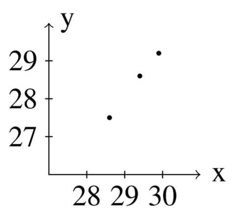
Then, we can find solutions for various values of n. Here are the solutions for values of n between 1 and 5 n=1:[25.020.0],n=2:[27.525.0],n=3:[28.7527.5] n=4:[29.37528.75],n=5:[29.68829.375]
Notice that as n increases, we approach the vector given by [2x0−y02x0−y0]=[2(20)−102(20)−10]=[3030]
These solutions are graphed in the following figure.
The following example demonstrates another system which exhibits some interesting behavior. When we graph the solutions, it is possible for the ordered pairs to spiral around the origin.
Suppose a dynamical system is of the form [x(n+1)y(n+1)]=[0.70.7−0.70.7][x(n)y(n)] Find solutions to the dynamical system for given initial conditions.
Solution
Let A=[0.70.7−0.70.7] To find solutions, we must diagonalize A. You can verify that the eigenvalues of A are complex and are given by λ1=.7+.7i and λ2=.7−.7i. The eigenvector for λ1=.7+.7i is [1i] and that the eigenvector for λ2=.7−.7i is [1−i]
Thus the matrix A can be written in the form [11i−i][.7+.7i00.7−.7i][12−12i1212i] and so, Vn=PDnP−1V0[x(n)y(n)]=[11i−i][(.7+.7i)n00(.7−.7i)n][12−12i1212i][x0y0]
The explicit solution is given by [x0(12(0.7−0.7i)n+12(0.7+0.7i)n)+y0(12i(0.7−0.7i)n−12i(0.7+0.7i)n)y0(12(0.7−0.7i)n+12(0.7+0.7i)n)−x0(12i(0.7−0.7i)n−12i(0.7+0.7i)n)]
Suppose the initial condition is [x0y0]=[1010] Then one obtains the following sequence of values which are graphed below by letting n=1,2,⋯,20
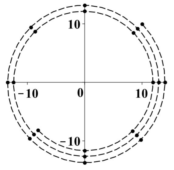
In this picture, the dots are the values and the dashed line is to help to picture what is happening.
These points are getting gradually closer to the origin, but they are circling the origin in the clockwise direction as they do so. As n increases, the vector [x(n)y(n)] approaches [00]
This type of behavior along with complex eigenvalues is typical of the deviations from an equilibrium point in the Lotka Volterra system of differential equations which is a famous model for predator-prey interactions. These differential equations are given by x′=x(a−by)y′=−y(c−dx) where a,b,c,d are positive constants. For example, you might have X be the population of moose and Y the population of wolves on an island.
Note that these equations make logical sense. The top says that the rate at which the moose population increases would be aX if there were no predators Y. However, this is modified by multiplying instead by (a−bY) because if there are predators, these will militate against the population of moose. The more predators there are, the more pronounced is this effect. As to the predator equation, you can see that the equations predict that if there are many prey around, then the rate of growth of the predators would seem to be high. However, this is modified by the term −cY because if there are many predators, there would be competition for the available food supply and this would tend to decrease Y′.
The behavior near an equilibrium point, which is a point where the right side of the differential equations equals zero, is of great interest. In this case, the equilibrium point is x=cd,y=ab Then one defines new variables according to the formula x+cd=x, y=y+ab In terms of these new variables, the differential equations become x′=(x+cd)(a−b(y+ab))y′=−(y+ab)(c−d(x+cd)) Multiplying out the right sides yields x′=−bxy−bcdyy′=dxy+abdx The interest is for x,y small and so these equations are essentially equal to x′=−bcdy, y′=abdx
Replace x′ with the difference quotient x(t+h)−x(t)h where h is a small positive number and y′ with a similar difference quotient. For example one could have h correspond to one day or even one hour. Thus, for h small enough, the following would seem to be a good approximation to the differential equations. x(t+h)=x(t)−hbcdyy(t+h)=y(t)+habdx Let 1,2,3,⋯ denote the ends of discrete intervals of time having length h chosen above. Then the above equations take the form [x(n+1)y(n+1)]=[1−hbcdhadb1][x(n)y(n)] Note that the eigenvalues of this matrix are always complex.
We are not interested in time intervals of length h for h very small. Instead, we are interested in much longer lengths of time. Thus, replacing the time interval with mh, [x(n+m)y(n+m)]=[1−hbcdhadb1]m[x(n)y(n)] For example, if m=2, you would have [x(n+2)y(n+2)]=[1−ach2−2bcdh2abdh1−ach2][x(n)y(n)] Note that most of the time, the eigenvalues of the new matrix will be complex.
You can also notice that the upper right corner will be negative by considering higher powers of the matrix. Thus letting 1,2,3,⋯ denote the ends of discrete intervals of time, the desired discrete dynamical system is of the form [x(n+1)y(n+1)]=[a−bcd][x(n)y(n)] where a,b,c,d are positive constants and the matrix will likely have complex eigenvalues because it is a power of a matrix which has complex eigenvalues.
You can see from the above discussion that if the eigenvalues of the matrix used to define the dynamical system are less than 1 in absolute value, then the origin is stable in the sense that as n→∞, the solution converges to the origin. If either eigenvalue is larger than 1 in absolute value, then the solutions to the dynamical system will usually be unbounded, unless the initial condition is chosen very carefully. The next example exhibits the case where one eigenvalue is larger than 1 and the other is smaller than 1.
The following example demonstrates a familiar concept as a dynamical system.
The Fibonacci sequence is the sequence given by 1,1,2,3,5,⋯ which is defined recursively in the form x(0)=1=x(1), x(n+2)=x(n+1)+x(n) Show how the Fibonacci Sequence can be considered a dynamical system.
Solution
This sequence is extremely important in the study of reproducing rabbits. It can be considered as a dynamical system as follows. Let y(n)=x(n+1). Then the above recurrence relation can be written as [x(n+1)y(n+1)]=[0111][x(n)y(n)], [x(0)y(0)]=[11]
Let A=[0111]
The eigenvalues of the matrix A are λ1=12−12√5 and λ2=12√5+12. The corresponding eigenvectors are, respectively, X1=[−12√5−121],X2=[12√5−121]
You can see from a short computation that one of the eigenvalues is smaller than 1 in absolute value while the other is larger than 1 in absolute value. Now, diagonalizing A gives us [12√5−12−12√5−1211]−1[0111][12√5−12−12√5−1211] =[12√5+120012−12√5]
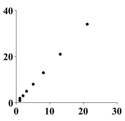
Then it follows that for a given initial condition, the solution to this dynamical system is of the form [x(n)y(n)]=[12√5−12−12√5−1211][(12√5+12)n00(12−12√5)n]⋅[15√5110√5+12−15√515√5(12√5−12)][11] It follows that x(n)=(12√5+12)n(110√5+12)+(12−12√5)n(12−110√5)
Here is a picture of the ordered pairs (x(n),y(n)) for n=0,1,⋯,n.
There is so much more that can be said about dynamical systems. It is a major topic of study in differential equations and what is given above is just an introduction.
The Matrix Exponential
The goal of this section is to use the concept of the matrix exponential to solve first order linear differential equations. We begin by proving the matrix exponential.
Suppose A is a diagonalizable matrix. Then the matrix exponential, written eA, can be easily defined. Recall that if D is a diagonal matrix, then P−1AP=D D is of the form [λ10⋱0λn] and it follows that Dm=[λm10⋱0λmn]
Since A is diagonalizable, A=PDP−1 and Am=PDmP−1
Recall why this is true. A=PDP−1 and so Am=m times⏞PDP−1PDP−1PDP−1⋯PDP−1=PDmP−1
We now will examine what is meant by the matrix exponental eA. Begin by formally writing the following power series for eA: eA=∞∑k=0Akk!=∞∑k=0PDkP−1k!=P(∞∑k=0Dkk!)P−1 If D is given above in (???), the above sum is of the form P(∞∑k=0[1k!λk10⋱01k!λkn])P−1 This can be rearranged as follows: eA=P[∑∞k=01k!λk10⋱0∑∞k=01k!λkn]P−1 =P[eλ10⋱0eλn]P−1
This justifies the following theorem.
Let A be a diagonalizable matrix, with eigenvalues λ1,...,λnand corresponding matrix of eigenvectors P. Then the matrix exponential, eA, is given by eA=P[eλ10⋱0eλn]P−1
Let A=[2−1−1121−112] Find eA.
Solution
The eigenvalues work out to be 1,2,3 and eigenvectors associated with these eigenvalues are [0−11]↔1,[−1−11]↔2,[−101]↔3 Then let D=[100020003],P=[0−1−1−1−10111] and so P−1=[101−1−1−1011]
Then the matrix exponential is eAt=[0−1−1−1−10111][e1000e2000e3][101−1−1−1011] [e2e2−e3e2−e3e2−ee2e2−e−e2+e−e2+e3−e2+e+e3]
The matrix exponential is a useful tool to solve autonomous systems of first order linear differential equations. These are equations which are of the form X′=AX,X(0)=C where A is a diagonalizable n×n matrix and C is a constant vector. X is a vector of functions in one variable, t: X=X(t)=[x1(t)x2(t)⋮xn(t)] Then X′ refers to the first derivative of X and is given by X′=X′(t)=[x′1(t)x′2(t)⋮x′n(t)],x′i(t)=the derivative ofxi(t)
Then it turns out that the solution to the above system of equations is X(t)=eAtC. To see this, suppose A is diagonalizable so that A=P[λ1⋱λn]P−1 Then eAt=P[eλ1t⋱eλnt]P−1 eAtC=P[eλ1t⋱eλnt]P−1C
Differentiating eAtC yields X′=(eAtC)′=P[λ1eλ1t⋱λneλnt]P−1C =P\left [ \begin{array}{ccc} \lambda _{1} & & \\ & \ddots & \\ & & \lambda _{n} \end{array} \right ] \left [ \begin{array}{ccc} e^{\lambda _{1}t} & & \\ & \ddots & \\ & & e^{\lambda _{n}t} \end{array} \right ] P^{-1}C\nonumber \begin{aligned} &=P\left [ \begin{array}{ccc} \lambda _{1} & & \\ & \ddots & \\ & & \lambda _{n} \end{array} \right ] P^{-1}P\left [ \begin{array}{ccc} e^{\lambda _{1}t} & & \\ & \ddots & \\ & & e^{\lambda _{n}t} \end{array} \right ] P^{-1}C \\ &=A\left( e^{At}C\right) = AX\end{aligned} Therefore X = X(t) = e^{At}C is a solution to X^{\prime }=AX.
To prove that X(0) = C if X(t) = e^{At}C: X(0) = e^{A0}C=P\left [ \begin{array}{ccc} 1 & & \\ & \ddots & \\ & & 1 \end{array} \right ] P^{-1}C=C\nonumber
Solve the initial value problem \left [ \begin{array}{c} x \\ y \end{array} \right ] ^{\prime }=\left [ \begin{array}{rr} 0 & -2 \\ 1 & 3 \end{array} \right ] \left [ \begin{array}{c} x \\ y \end{array} \right ] ,\ \left [ \begin{array}{c} x(0)\\ y(0) \end{array} \right ] =\left [ \begin{array}{c} 1 \\ 1 \end{array} \right ]\nonumber
Solution
The matrix is diagonalizable and can be written as \begin{aligned} A &= PDP^{-1} \\ \left [ \begin{array}{rr} 0 & -2 \\ 1 & 3 \end{array} \right ] &=\left [ \begin{array}{rr} 1 & 1 \\ -\frac{1}{2} & -1 \end{array} \right ] \left [ \begin{array}{rr} 1 & 0 \\ 0 & 2 \end{array} \right ] \left [ \begin{array}{rr} 2 & 2 \\ -1 & -2 \end{array} \right ]\end{aligned} Therefore, the matrix exponential is of the form e^{At} = \left [ \begin{array}{rr} 1 & 1 \\ -\frac{1}{2} & -1 \end{array} \right ] \left [ \begin{array}{cc} e^{t} & 0 \\ 0 & e^{2t} \end{array} \right ] \left [ \begin{array}{rr} 2 & 2 \\ -1 & -2 \end{array} \right ]\nonumber The solution to the initial value problem is \begin{aligned} X(t) &= e^{At}C \\ \left [ \begin{array}{c} x\left( t\right) \\ y\left( t\right) \end{array} \right ] &= \left [ \begin{array}{rr} 1 & 1 \\ -\frac{1}{2} & -1 \end{array} \right ] \left [ \begin{array}{cc} e^{t} & 0 \\ 0 & e^{2t} \end{array} \right ] \left [ \begin{array}{rr} 2 & 2 \\ -1 & -2 \end{array} \right ] \left [ \begin{array}{c} 1 \\ 1 \end{array} \right ] \\ &=\left [ \begin{array}{c} 4e^{t}-3e^{2t} \\ 3e^{2t}-2e^{t} \end{array} \right ]\end{aligned} We can check that this works: \begin{aligned} \left [ \begin{array}{c} x\left( 0\right) \\ y\left( 0\right) \end{array} \right ] &= \left [ \begin{array}{c} 4e^{0}-3e^{2(0)} \\ 3e^{2(0)}-2e^{0} \end{array} \right ] \\ &= \left [ \begin{array}{c} 1 \\ 1 \end{array} \right ]\end{aligned}
Lastly, X^{\prime} = \left [ \begin{array}{c} 4e^{t}-3e^{2t} \\ 3e^{2t}-2e^{t} \end{array} \right ] ^{\prime }=\left [ \begin{array}{c} 4e^{t}-6e^{2t} \\ 6e^{2t}-2e^{t} \end{array} \right ]\nonumber and AX = \left [ \begin{array}{rr} 0 & -2 \\ 1 & 3 \end{array} \right ] \left [ \begin{array}{c} 4e^{t}-3e^{2t} \\ 3e^{2t}-2e^{t} \end{array} \right ] =\left [ \begin{array}{c} 4e^{t}-6e^{2t} \\ 6e^{2t}-2e^{t} \end{array} \right ]\nonumber which is the same thing. Thus this is the solution to the initial value problem.