1.4: Existence and Uniqueness of Solutions

Learning Objectives

• T/F: It is possible for a linear system to have exactly 5 solutions.
• T/F: A variable that corresponds to a leading 1 is “free.”
• How can one tell what kind of solution a linear system of equations has?
• Give an example (different from those given in the text) of a 2 equation, 2 unknown linear system that is not consistent.
• T/F: A particular solution for a linear system with infinite solutions can be found by arbitrarily picking values for the free variables.

So far, whenever we have solved a system of linear equations, we have always found exactly one solution. This is not always the case; we will find in this section that some systems do not have a solution, and others have more than one.

We start with a very simple example. Consider the following linear system: $$x-y=0. \nonumber$$ There are obviously infinite solutions to this system; as long as $x=y$, we have a solution. We can picture all of these solutions by thinking of the graph of the equation $y=x$ on the traditional $x,y$ coordinate plane.

Let’s continue this visual aspect of considering solutions to linear systems. Consider the system $$\begin{align}\begin{aligned} x+y&=2\\ x-y&=0. \end{aligned}\end{align} \nonumber$$ Each of these equations can be viewed as lines in the coordinate plane, and since their slopes are different, we know they will intersect somewhere (see Figure $\PageIndex{1}$(a)). In this example, they intersect at the point $(1,1)$ – that is, when $x=1$ and $y=1$, both equations are satisfied and we have a solution to our linear system. Since this is the only place the two lines intersect, this is the only solution.

Now consider the linear system $$\begin{align}\begin{aligned} x+y&=1\\2x+2y&=2.\end{aligned}\end{align} \nonumber$$ It is clear that while we have two equations, they are essentially the same equation; the second is just a multiple of the first. Therefore, when we graph the two equations, we are graphing the same line twice (see Figure $\PageIndex{1}$(b); the thicker line is used to represent drawing the line twice). In this case, we have an infinite solution set, just as if we only had the one equation $x+y=1$. We often write the solution as $x=1-y$ to demonstrate that $y$ can be any real number, and $x$ is determined once we pick a value for $y$.

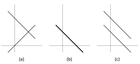
Figure $\PageIndex{1}$: The three possibilities for two linear equations with two unknowns.

Finally, consider the linear system $$\begin{align}\begin{aligned} x+y&=1\\x+y&=2.\end{aligned}\end{align} \nonumber$$ We should immediately spot a problem with this system; if the sum of $x$ and $y$ is 1, how can it also be 2? There is no solution to such a problem; this linear system has no solution. We can visualize this situation in Figure $\PageIndex{1}$ (c); the two lines are parallel and never intersect.

If we were to consider a linear system with three equations and two unknowns, we could visualize the solution by graphing the corresponding three lines. We can picture that perhaps all three lines would meet at one point, giving exactly 1 solution; perhaps all three equations describe the same line, giving an infinite number of solutions; perhaps we have different lines, but they do not all meet at the same point, giving no solution. We further visualize similar situations with, say, 20 equations with two variables.

While it becomes harder to visualize when we add variables, no matter how many equations and variables we have, solutions to linear equations always come in one of three forms: exactly one solution, infinite solutions, or no solution. This is a fact that we will not prove here, but it deserves to be stated.

Theorem $\PageIndex{1}$

Solution Forms of Linear Systems

Every linear system of equations has exactly one solution, infinite solutions, or no solution.

This leads us to a definition. Here we don’t differentiate between having one solution and infinite solutions, but rather just whether or not a solution exists.

Definition: Consistent and Inconsistent Linear Systems

A system of linear equations is consistent if it has a solution (perhaps more than one). A linear system is inconsistent if it does not have a solution.

How can we tell what kind of solution (if one exists) a given system of linear equations has? The answer to this question lies with properly understanding the reduced row echelon form of a matrix. To discover what the solution is to a linear system, we first put the matrix into reduced row echelon form and then interpret that form properly.

Before we start with a simple example, let us make a note about finding the reduced row echelon form of a matrix.

Note

In the previous section, we learned how to find the reduced row echelon form of a matrix using Gaussian elimination – by hand. We need to know how to do this; understanding the process has benefits. However, actually executing the process by hand for every problem is not usually beneficial. In fact, with large systems, computing the reduced row echelon form by hand is effectively impossible. Our main concern is what “the rref” is, not what exact steps were used to arrive there. Therefore, the reader is encouraged to employ some form of technology to find the reduced row echelon form. Computer programs such as Mathematica, MATLAB, Maple, and Derive can be used; many handheld calculators (such as Texas Instruments calculators) will perform these calculations very quickly.

As a general rule, when we are learning a new technique, it is best to not use technology to aid us. This helps us learn not only the technique but some of its “inner workings.” We can then use technology once we have mastered the technique and are now learning how to use it to solve problems.

From here on out, in our examples, when we need the reduced row echelon form of a matrix, we will not show the steps involved. Rather, we will give the initial matrix, then immediately give the reduced row echelon form of the matrix. We trust that the reader can verify the accuracy of this form by both performing the necessary steps by hand or utilizing some technology to do it for them.

Our first example explores officially a quick example used in the introduction of this section.

Example $\PageIndex{1}$

Find the solution to the linear system

$$\begin{array}{ccccc} x_1 & +& x_2 & = & 1\\ 2x_1 & + & 2x_2 & = &2\end{array} . \nonumber$$

Solution

Create the corresponding augmented matrix, and then put the matrix into reduced row echelon form.

$$\left[\begin{array}{ccc}{1}&{1}&{1}\\{2}&{2}&{2}\end{array}\right]\qquad\overrightarrow{\text{rref}}\qquad\left[\begin{array}{ccc}{1}&{1}&{1}\\{0}&{0}&{0}\end{array}\right] \nonumber$$

Now convert the reduced matrix back into equations. In this case, we only have one equation, $$x_1+x_2=1 \nonumber$$ or, equivalently, $$\begin{align}\begin{aligned} x_1 &=1-x_2\\ x_2&\text{ is free}. \end{aligned}\end{align} \nonumber$$

We have just introduced a new term, the word free. It is used to stress that idea that $x_2$ can take on any value; we are “free” to choose any value for $x_2$. Once this value is chosen, the value of $x_1$ is determined. We have infinite choices for the value of $x_2$, so therefore we have infinite solutions.

For example, if we set $x_2 = 0$, then $x_1 = 1$; if we set $x_2 = 5$, then $x_1 = -4$.

Let’s try another example, one that uses more variables.

Example $\PageIndex{2}$

Find the solution to the linear system $$\begin{array}{ccccccc} & &x_2&-&x_3&=&3\\ x_1& & &+&2x_3&=&2\\ &&-3x_2&+&3x_3&=&-9\\ \end{array}. \nonumber$$

Solution

To find the solution, put the corresponding matrix into reduced row echelon form.

$$\left[\begin{array}{cccc}{0}&{1}&{-1}&{3}\\{1}&{0}&{2}&{2}\\{0}&{-3}&{3}&{-9}\end{array}\right]\qquad\overrightarrow{\text{rref}}\qquad\left[\begin{array}{cccc}{1}&{0}&{2}&{2}\\{0}&{1}&{-1}&{3}\\{0}&{0}&{0}&{0}\end{array}\right] \nonumber$$

Now convert this reduced matrix back into equations. We have $$\begin{align}\begin{aligned} x_1 + 2x_3 &= 2 \\ x_2-x_3&=3 \end{aligned}\end{align} \nonumber$$ or, equivalently, $$\begin{align}\begin{aligned} x_1 &= 2-2x_3 \\ x_2&=3+x_3\\x_3&\text{ is free.} \end{aligned}\end{align} \nonumber$$

These two equations tell us that the values of $x_1$ and $x_2$ depend on what $x_3$ is. As we saw before, there is no restriction on what $x_3$ must be; it is “free” to take on the value of any real number. Once $x_3$ is chosen, we have a solution. Since we have infinite choices for the value of $x_3$, we have infinite solutions.

As examples, $x_1 = 2$, $x_2 = 3$, $x_3 = 0$ is one solution; $x_1 = -2$, $x_2 = 5$, $x_3 = 2$ is another solution. Try plugging these values back into the original equations to verify that these indeed are solutions. (By the way, since infinite solutions exist, this system of equations is consistent.)

In the two previous examples we have used the word “free” to describe certain variables. What exactly is a free variable? How do we recognize which variables are free and which are not?

Look back to the reduced matrix in Example $\PageIndex{1}$. Notice that there is only one leading 1 in that matrix, and that leading 1 corresponded to the $x_1$ variable. That told us that $x_1$ was not a free variable; since $x_2$ did not correspond to a leading 1, it was a free variable.

Look also at the reduced matrix in Example $\PageIndex{2}$. There were two leading 1s in that matrix; one corresponded to $x_1$ and the other to $x_2$. This meant that $x_1$ and $x_2$ were not free variables; since there was not a leading 1 that corresponded to $x_3$, it was a free variable.

We formally define this and a few other terms in this following definition.

Definition: Dependent and Independent Variables

Consider the reduced row echelon form of an augmented matrix of a linear system of equations. Then:

a variable that corresponds to a leading 1 is a basic, or dependent, variable, and

a variable that does not correspond to a leading 1 is a free, or independent, variable.

One can probably see that “free” and “independent” are relatively synonymous. It follows that if a variable is not independent, it must be dependent; the word “basic” comes from connections to other areas of mathematics that we won’t explore here.

These definitions help us understand when a consistent system of linear equations will have infinite solutions. If there are no free variables, then there is exactly one solution; if there are any free variables, there are infinite solutions.

Key Idea $\PageIndex{1}$: Consistent Solution Types

A consistent linear system of equations will have exactly one solution if and only if there is a leading 1 for each variable in the system.

If a consistent linear system of equations has a free variable, it has infinite solutions.

If a consistent linear system has more variables than leading 1s, then the system will have infinite solutions.

A consistent linear system with more variables than equations will always have infinite solutions.

Note

Key Idea $\PageIndex{1}$ applies only to consistent systems. If a system is inconsistent, then no solution exists and talking about free and basic variables is meaningless.

When a consistent system has only one solution, each equation that comes from the reduced row echelon form of the corresponding augmented matrix will contain exactly one variable. If the consistent system has infinite solutions, then there will be at least one equation coming from the reduced row echelon form that contains more than one variable. The “first” variable will be the basic (or dependent) variable; all others will be free variables.

We have now seen examples of consistent systems with exactly one solution and others with infinite solutions. How will we recognize that a system is inconsistent? Let’s find out through an example.

Example $\PageIndex{3}$

Find the solution to the linear system $$\begin{array}{ccccccc} x_1&+&x_2&+&x_3&=&1\\ x_1&+&2x_2&+&x_3&=&2\\ 2x_1&+&3x_2&+&2x_3&=&0\\ \end{array}. \nonumber$$

Solution

We start by putting the corresponding matrix into reduced row echelon form.

$$\left[\begin{array}{cccc}{1}&{1}&{1}&{1}\\{1}&{2}&{1}&{2}\\{2}&{3}&{2}&{0}\end{array}\right]\qquad\overrightarrow{\text{rref}}\qquad\left[\begin{array}{cccc}{1}&{0}&{1}&{0}\\{0}&{1}&{0}&{0}\\{0}&{0}&{0}&{1}\end{array}\right] \nonumber$$

Now let us take the reduced matrix and write out the corresponding equations. The first two rows give us the equations $$\begin{align}\begin{aligned} x_1+x_3&=0\\ x_2 &= 0.\\ \end{aligned}\end{align} \nonumber$$ So far, so good. However the last row gives us the equation $$0x_1+0x_2+0x_3 = 1 \nonumber$$ or, more concisely, $0=1$. Obviously, this is not true; we have reached a contradiction. Therefore, no solution exists; this system is inconsistent.

In previous sections we have only encountered linear systems with unique solutions (exactly one solution). Now we have seen three more examples with different solution types. The first two examples in this section had infinite solutions, and the third had no solution. How can we tell if a system is inconsistent?

A linear system will be inconsistent only when it implies that 0 equals 1. We can tell if a linear system implies this by putting its corresponding augmented matrix into reduced row echelon form. If we have any row where all entries are 0 except for the entry in the last column, then the system implies 0=1. More succinctly, if we have a leading 1 in the last column of an augmented matrix, then the linear system has no solution.

Key Idea $\PageIndex{2}$: Inconsistent Systems of Linear Equations

A system of linear equations is inconsistent if the reduced row echelon form of its corresponding augmented matrix has a leading 1 in the last column.

Example $\PageIndex{4}$

Confirm that the linear system $$\begin{array}{ccccc} x&+&y&=&0 \\2x&+&2y&=&4 \end{array} \nonumber$$ has no solution.

Solution

We can verify that this system has no solution in two ways. First, let’s just think about it. If $x+y=0$, then it stands to reason, by multiplying both sides of this equation by 2, that $2x+2y = 0$. However, the second equation of our system says that $2x+2y= 4$. Since $0\neq 4$, we have a contradiction and hence our system has no solution. (We cannot possibly pick values for $x$ and $y$ so that $2x+2y$ equals both 0 and 4.)

Now let us confirm this using the prescribed technique from above. The reduced row echelon form of the corresponding augmented matrix is

$$\left[\begin{array}{ccc}{1}&{1}&{0}\\{0}&{0}&{1}\end{array}\right] \nonumber$$

We have a leading 1 in the last column, so therefore the system is inconsistent.

Let’s summarize what we have learned up to this point. Consider the reduced row echelon form of the augmented matrix of a system of linear equations.$^{1}$ If there is a leading 1 in the last column, the system has no solution. Otherwise, if there is a leading 1 for each variable, then there is exactly one solution; otherwise (i.e., there are free variables) there are infinite solutions.

Systems with exactly one solution or no solution are the easiest to deal with; systems with infinite solutions are a bit harder to deal with. Therefore, we’ll do a little more practice. First, a definition: if there are infinite solutions, what do we call one of those infinite solutions?

Definition: Particular Solution

Consider a linear system of equations with infinite solutions. A particular solution is one solution out of the infinite set of possible solutions.

The easiest way to find a particular solution is to pick values for the free variables which then determines the values of the dependent variables. Again, more practice is called for.

Example $\PageIndex{5}$

Give the solution to a linear system whose augmented matrix in reduced row echelon form is

$$\left[\begin{array}{ccccc}{1}&{-1}&{0}&{2}&{4}\\{0}&{0}&{1}&{-3}&{7}\\{0}&{0}&{0}&{0}&{0}\end{array}\right] \nonumber$$

and give two particular solutions.

Solution

We can essentially ignore the third row; it does not divulge any information about the solution.$^{2}$ The first and second rows can be rewritten as the following equations: $$\begin{align}\begin{aligned} x_1 - x_2 + 2x_4 &=4 \\ x_3 - 3x_4 &= 7. \\ \end{aligned}\end{align} \nonumber$$ Notice how the variables $x_1$ and $x_3$ correspond to the leading 1s of the given matrix. Therefore $x_1$ and $x_3$ are dependent variables; all other variables (in this case, $x_2$ and $x_4$) are free variables.

We generally write our solution with the dependent variables on the left and independent variables and constants on the right. It is also a good practice to acknowledge the fact that our free variables are, in fact, free. So our final solution would look something like $$\begin{align}\begin{aligned} x_1 &= 4 +x_2 - 2x_4 \\ x_2 & \text{ is free} \\ x_3 &= 7+3x_4 \\ x_4 & \text{ is free}.\end{aligned}\end{align} \nonumber$$

To find particular solutions, choose values for our free variables. There is no “right” way of doing this; we are “free” to choose whatever we wish.

By setting $x_2 = 0 = x_4$, we have the solution $x_1 = 4$, $x_2 = 0$, $x_3 = 7$, $x_4 = 0$. By setting $x_2 = 1$ and $x_4 = -5$, we have the solution $x_1 = 15$, $x_2 = 1$, $x_3 = -8$, $x_4 = -5$. It is easier to read this when are variables are listed vertically, so we repeat these solutions:

One particular solution is:

$$\begin{align}\begin{aligned} x_1 &= 4\\ x_2 &=0 \\ x_3 &= 7 \\ x_4 &= 0. \end{aligned}\end{align} \nonumber$$

Another particular solution is:

$$\begin{align}\begin{aligned} x_1 &= 15\\ x_2 &=1 \\ x_3 &= -8 \\ x_4 &= -5. \end{aligned}\end{align} \nonumber$$

Example $\PageIndex{6}$

Find the solution to a linear system whose augmented matrix in reduced row echelon form is

$$\left[\begin{array}{ccccc}{1}&{0}&{0}&{2}&{3}\\{0}&{1}&{0}&{4}&{5}\end{array}\right] \nonumber$$

and give two particular solutions.

Solution

Converting the two rows into equations we have $$\begin{align}\begin{aligned} x_1 + 2x_4 &= 3 \\ x_2 + 4x_4&=5.\\ \end{aligned}\end{align} \nonumber$$

We see that $x_1$ and $x_2$ are our dependent variables, for they correspond to the leading 1s. Therefore, $x_3$ and $x_4$ are independent variables. This situation feels a little unusual,$^{3}$ for $x_3$ doesn’t appear in any of the equations above, but cannot overlook it; it is still a free variable since there is not a leading 1 that corresponds to it. We write our solution as: $$\begin{align}\begin{aligned} x_1 &= 3-2x_4 \\ x_2 &=5-4x_4 \\ x_3 & \text{ is free} \\ x_4 & \text{ is free}. \\ \end{aligned}\end{align} \nonumber$$

To find two particular solutions, we pick values for our free variables. Again, there is no “right” way of doing this (in fact, there are $\ldots$ infinite ways of doing this) so we give only an example here.

One particular solution is:

$$\begin{align}\begin{aligned} x_1 &= 3\\ x_2 &=5 \\ x_3 &= 1000 \\ x_4 &= 0. \end{aligned}\end{align} \nonumber$$

Another particular solution is:

$$\begin{align}\begin{aligned} x_1 &= 3-2\pi\\ x_2 &=5-4\pi \\ x_3 &= e^2 \\ x_4 &= \pi. \end{aligned}\end{align} \nonumber$$

(In the second particular solution we picked “unusual” values for $x_3$ and $x_4$ just to highlight the fact that we can.)

Example $\PageIndex{7}$

Find the solution to the linear system $$\begin{array}{ccccccc}x_1&+&x_2&+&x_3&=&5\\x_1&-&x_2&+&x_3&=&3\\ \end{array} \nonumber$$ and give two particular solutions.

Solution

The corresponding augmented matrix and its reduced row echelon form are given below.

$$\left[\begin{array}{cccc}{1}&{1}&{1}&{5}\\{1}&{-1}&{1}&{3}\end{array}\right]\qquad\overrightarrow{\text{rref}}\qquad\left[\begin{array}{cccc}{1}&{0}&{1}&{4}\\{0}&{1}&{0}&{1}\end{array}\right] \nonumber$$

Converting these two rows into equations, we have $$\begin{align}\begin{aligned} x_1+x_3&=4\\x_2&=1\\ \end{aligned}\end{align} \nonumber$$ giving us the solution $$\begin{align}\begin{aligned} x_1&= 4-x_3\\x_2&=1\\x_3 &\text{ is free}.\\ \end{aligned}\end{align} \nonumber$$

Once again, we get a bit of an “unusual” solution; while $x_2$ is a dependent variable, it does not depend on any free variable; instead, it is always 1. (We can think of it as depending on the value of 1.) By picking two values for $x_3$, we get two particular solutions.

One particular solution is:

$$\begin{align}\begin{aligned} x_1 &= 4\\ x_2 &=1 \\ x_3 &= 0 . \end{aligned}\end{align} \nonumber$$

Another particular solution is:

$$\begin{align}\begin{aligned} x_1 &= 3\\ x_2 &=1 \\ x_3 &= 1 . \end{aligned}\end{align} \nonumber$$

The constants and coefficients of a matrix work together to determine whether a given system of linear equations has one, infinite, or no solution. The concept will be fleshed out more in later chapters, but in short, the coefficients determine whether a matrix will have exactly one solution or not. In the “or not” case, the constants determine whether or not infinite solutions or no solution exists. (So if a given linear system has exactly one solution, it will always have exactly one solution even if the constants are changed.) Let’s look at an example to get an idea of how the values of constants and coefficients work together to determine the solution type.

Example $\PageIndex{8}$

For what values of $k$ will the given system have exactly one solution, infinite solutions, or no solution? $$\begin{array}{ccccc}x_1&+&2x_2&=&3\\ 3x_1&+&kx_2&=&9\end{array} \nonumber$$

Solution

We answer this question by forming the augmented matrix and starting the process of putting it into reduced row echelon form. Below we see the augmented matrix and one elementary row operation that starts the Gaussian elimination process.

$$\left[\begin{array}{ccc}{1}&{2}&{3}\\{3}&{k}&{9}\end{array}\right]\qquad\overrightarrow{-3R_{1}+R_{2}\to R_{2}}\qquad\left[\begin{array}{ccc}{1}&{2}&{3}\\{0}&{k-6}&{0}\end{array}\right] \nonumber$$

This is as far as we need to go. In looking at the second row, we see that if $k=6$, then that row contains only zeros and $x_2$ is a free variable; we have infinite solutions. If $k\neq 6$, then our next step would be to make that second row, second column entry a leading one. We don’t particularly care about the solution, only that we would have exactly one as both $x_1$ and $x_2$ would correspond to a leading one and hence be dependent variables.

Our final analysis is then this. If $k\neq 6$, there is exactly one solution; if $k=6$, there are infinite solutions. In this example, it is not possible to have no solutions.

As an extension of the previous example, consider the similar augmented matrix where the constant 9 is replaced with a 10. Performing the same elementary row operation gives

$$\left[\begin{array}{ccc}{1}&{2}&{3}\\{3}&{k}&{10}\end{array}\right]\qquad\overrightarrow{-3R_{1}+R_{2}\to R_{2}}\qquad\left[\begin{array}{ccc}{1}&{2}&{3}\\{0}&{k-6}&{1}\end{array}\right] \nonumber$$

As in the previous example, if $k\neq6$, we can make the second row, second column entry a leading one and hence we have one solution. However, if $k=6$, then our last row is $[0\ 0\ 1]$, meaning we have no solution.

We have been studying the solutions to linear systems mostly in an “academic” setting; we have been solving systems for the sake of solving systems. In the next section, we’ll look at situations which create linear systems that need solving (i.e., “word problems”).

Footnotes

[1] That sure seems like a mouthful in and of itself. However, it boils down to “look at the reduced form of the usual matrix.”

[2] Then why include it? Rows of zeros sometimes appear “unexpectedly” in matrices after they have been put in reduced row echelon form. When this happens, we do learn something; it means that at least one equation was a combination of some of the others.

[3] What kind of situation would lead to a column of all zeros? To have such a column, the original matrix needed to have a column of all zeros, meaning that while we acknowledged the existence of a certain variable, we never actually used it in any equation. In practical terms, we could respond by removing the corresponding column from the matrix and just keep in mind that that variable is free. In very large systems, it might be hard to determine whether or not a variable is actually used and one would not worry about it.

When we learn about s and s, we will see that under certain circumstances this situation arises. In those cases we leave the variable in the system just to remind ourselves that it is there.