5.1: Transformations of the Cartesian Plane

Last updated
Save as PDF

Page ID: 63402

$ \newcommand{\vecs}[1]{\overset { \scriptstyle \rightharpoonup} {\mathbf{#1}} } $ $ \newcommand{\vecd}[1]{\overset{-\!-\!\rightharpoonup}{\vphantom{a}\smash {#1}}} $$\newcommand{\id}{\mathrm{id}}$ $ \newcommand{\Span}{\mathrm{span}}$ $ \newcommand{\kernel}{\mathrm{null}\,}$ $ \newcommand{\range}{\mathrm{range}\,}$ $ \newcommand{\RealPart}{\mathrm{Re}}$ $ \newcommand{\ImaginaryPart}{\mathrm{Im}}$ $ \newcommand{\Argument}{\mathrm{Arg}}$ $ \newcommand{\norm}[1]{\| #1 \|}$ $ \newcommand{\inner}[2]{\langle #1, #2 \rangle}$ $ \newcommand{\Span}{\mathrm{span}}$ $\newcommand{\id}{\mathrm{id}}$ $ \newcommand{\Span}{\mathrm{span}}$ $ \newcommand{\kernel}{\mathrm{null}\,}$ $ \newcommand{\range}{\mathrm{range}\,}$ $ \newcommand{\RealPart}{\mathrm{Re}}$ $ \newcommand{\ImaginaryPart}{\mathrm{Im}}$ $ \newcommand{\Argument}{\mathrm{Arg}}$ $ \newcommand{\norm}[1]{\| #1 \|}$ $ \newcommand{\inner}[2]{\langle #1, #2 \rangle}$ $ \newcommand{\Span}{\mathrm{span}}$$\newcommand{\AA}{\unicode[.8,0]{x212B}}$

Learning Objectives

To understand how the Cartesian plane is affected by multiplication by a matrix, it helps to study how what is affected?
Transforming the Cartesian plane through matrix multiplication transforms straight lines into what kind of lines?
T/F: If one draws a picture of a sheep on the Cartesian plane, then transformed the plane using the matrix
\[\left[\begin{array}{cc}{-1}&{0}\\{0}&{1}\end{array}\right], \nonumber \]
one could say that the sheep was “sheared.

We studied in Section 2.3 how to visualize vectors and how certain matrix arithmetic operations can be graphically represented. We limited our visual understanding of matrix multiplication to graphing a vector, multiplying it by a matrix, then graphing the resulting vector. In this section we’ll explore these multiplication ideas in greater depth. Instead of multiplying individual vectors by a matrix $A$, we’ll study what happens when we multiply every vector in the Cartesian plans by $A$.$^{1}$

Because of the Distributive Property, demonstrated way back in Example 2.3.11, we can say that the Cartesian plane will be transformed in a very nice, predictable way. Straight lines will be transformed into other straight lines (and they won’t become curvy, or jagged, or broken). Curved lines will be transformed into other curved lines (perhaps the curve will become “straight,” but it won’t become jagged or broken).

One way of studying how the whole Cartesian plane is affected by multiplication by a matrix $A$ is to study how the unit square is affected. The unit square is the square with corners at the points $(0,0)$, $(1,0)$, $(1,1)$, and $(0,1)$. Each corner can be represented by the vector that points to it; multiply each of these vectors by $A$ and we can get an idea of how $A$ affects the whole Cartesian plane.

Let’s try an example.

Example $\PageIndex{1}$

Plot the vectors of the unit square before and after they have been multiplied by $A$, where

\[A=\left[\begin{array}{cc}{1}&{4}\\{2}&{3}\end{array}\right]. \nonumber \]

Solution

The four corners of the unit square can be represented by the vectors

\[\left[\begin{array}{c}{0}\\{0}\end{array}\right],\quad\left[\begin{array}{c}{1}\\{0}\end{array}\right],\quad\left[\begin{array}{c}{1}\\{1}\end{array}\right],\quad\left[\begin{array}{c}{0}\\{1}\end{array}\right]. \nonumber \]

Multiplying each by $A$ gives the vectors

\[\left[\begin{array}{c}{0}\\{0}\end{array}\right],\quad\left[\begin{array}{c}{1}\\{2}\end{array}\right],\quad\left[\begin{array}{c}{5}\\{5}\end{array}\right],\quad\left[\begin{array}{c}{4}\\{3}\end{array}\right]. \nonumber \]

respectively.

(Hint: one way of using your calculator to do this for you quickly is to make a $2\times 4$ matrix whose columns are each of these vectors. In this case, create a matrix

\[B=\left[\begin{array}{cccc}{0}&{1}&{1}&{0}\\{0}&{0}&{1}&{1}\end{array}\right]. \nonumber \]

Then multiply $B$ by $A$ and read off the transformed vectors from the respective columns:

\[AB=\left[\begin{array}{cccc}{0}&{1}&{5}&{4}\\{0}&{2}&{5}&{3}\end{array}\right]. \nonumber \]

This saves time, especially if you do a similar procedure for multiple matrices $A$. Of course, we can save more time by skipping the first column; since it is the column of zeros, it will stay the column of zeros after multiplication by $A$.)

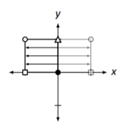
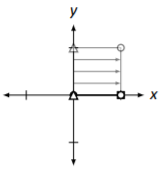
The unit square and its transformation are graphed in Figure $\PageIndex{1}$, where the shaped vertices correspond to each other across the two graphs. Note how the square got turned into some sort of quadrilateral (it’s actually a parallelogram). A really interesting thing is how the triangular and square vertices seem to have changed places – it is as though the square, in addition to being stretched out of shape, was flipped.

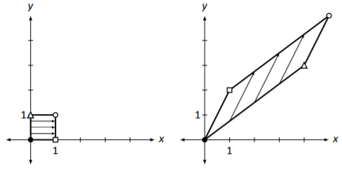
$clipboard_ee653c51c10d0511e537d75cd4beaa05c.png$

Figure $\PageIndex{1}$: Transforming the unit square by matrix multiplication in Example $\PageIndex{1}$.

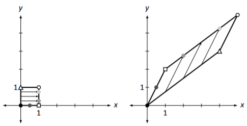
$clipboard_ebdb152c9ef703017e6ca3a101d7998db.png$

Figure $\PageIndex{2}$: Emphasizing straight lines going to straight lines in Example $\PageIndex{1}$.

To stress how “straight lines get transformed to straight lines,” consider Figure $\PageIndex{2}$. Here, the unit square has some additional points drawn on it which correspond to the shaded dots on the transformed parallelogram. Note how relative distances are also preserved; the dot halfway between the black and square dots is transformed to a position along the line, halfway between the black and square dots.

Much more can be said about this example. Before we delve into this, though, let’s try one more example.

Example $\PageIndex{2}$

Plot the transformed unit square after it has been transformed by $A$, where

\[A=\left[\begin{array}{cc}{0}&{-1}\\{1}&{0}\end{array}\right]. \nonumber \]

Solution

We’ll put the vectors that correspond to each corner in a matrix $B$ as before and then multiply it on the left by $A$. Doing so gives:

\[\begin{align}\begin{aligned}AB&=\left[\begin{array}{cc}{0}&{-1}\\{1}&{0}\end{array}\right]\left[\begin{array}{cccc}{0}&{1}&{1}&{0}\\{0}&{0}&{1}&{1}\end{array}\right] \\ &=\left[\begin{array}{cccc}{0}&{0}&{-1}&{-1}\\{0}&{1}&{1}&{0}\end{array}\right]\end{aligned}\end{align} \nonumber \]

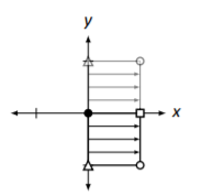
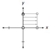
In Figure $\PageIndex{3}$ the unit square is again drawn along with its transformation by $A$.

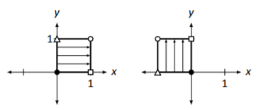
$clipboard_ed312dd7935f512d62a7b13a285c3fa9f.png$

Figure $\PageIndex{3}$: Transforming the unit square by matrix multiplication in Example $\PageIndex{2}$.

Make note of how the square moved. It did not simply “slide” to the left;$^{2}$ nor did it “flip” across the $y$ axis. Rather, it was rotated counterclockwise about the origin $90^\circ$. In a rotation, the shape of an object does not change; in our example, the square remained a square of the same size.

We have broached the topic of how the Cartesian plane can be transformed via multiplication by a $2\times 2$ matrix $A$. We have seen two examples so far, and our intuition as to how the plane is changed has been informed only by seeing how the unit square changes. Let’s explore this further by investigating two questions:

Suppose we want to transform the Cartesian plane in a known way (for instance, we may want to rotate the plane counterclockwise $180^\circ$). How do we find the matrix (if one even exists) which performs this transformation?
How does knowing how the unit square is transformed really help in understanding how the entire plane is transformed?

These questions are closely related, and as we answer one, we will help answer the other.

To get started with the first question, look back at Examples $\PageIndex{1}$ and $\PageIndex{2}$ and consider again how the unit square was transformed. In particular, is there any correlation between where the vertices ended up and the matrix $A$?

If you are just reading on, and haven’t actually gone back and looked at the examples, go back now and try to make some sort of connection. Otherwise – you may have noted some of the following things:

The zero vector ($\vec{0}$, the “black” corner) never moved. That makes sense, though; $A\vec{0}=\vec{0}$.
The “square” corner, i.e., the corner corresponding to the vector $\left[\begin{array}{c}{1}\\{0}\end{array}\right]$, is always transformed to the vector in the first column of $A$!
Likewise, the “triangular” corner, i.e., the corner corresponding to the vector $\left[\begin{array}{c}{0}\\{1}\end{array}\right]$, is always transformed to the vector in the second column of $A$!$^{3}$
The “white dot” corner is always transformed to the sum of the two column vectors of $A$.$^{4}$

Let’s now take the time to understand these four points. The first point should be clear; $\vec{0}$ will always be transformed to $\vec{0}$ via matrix multiplication. (Hence the hint in the middle of Example $\PageIndex{1}$, where we are told that we can ignore entering in the column of zeros in the matrix $B$.)

We can understand the second and third points simultaneously. Let

\[A=\left[\begin{array}{cc}{a}&{b}\\{c}&{d}\end{array}\right],\quad\vec{e_{1}}=\left[\begin{array}{c}{1}\\{0}\end{array}\right]\quad\text{and}\quad\vec{e_{2}}=\left[\begin{array}{c}{0}\\{1}\end{array}\right]. \nonumber \]

What are $A\vec{e_{1}}$ and $A\vec{e_{2}}$?

\[\begin{align}\begin{aligned}A\vec{e_{1}}&=\left[\begin{array}{cc}{a}&{b}\\{c}&{d}\end{array}\right]\left[\begin{array}{c}{1}\\{0}\end{array}\right] \\ &=\left[\begin{array}{c}{a}\\{c}\end{array}\right]\end{aligned}\end{align} \nonumber \]

\[\begin{align}\begin{aligned}A\vec{e_{2}}&=\left[\begin{array}{cc}{a}&{b}\\{c}&{d}\end{array}\right]\left[\begin{array}{c}{0}\\{1}\end{array}\right] \\ &=\left[\begin{array}{c}{b}\\{d}\end{array}\right]\end{aligned}\end{align} \nonumber \]

So by mere mechanics of matrix multiplication, the square corner $\vec{e_{1}}$ is transformed to the first column of $A$, and the triangular corner $\vec{e_{2}}$ is transformed to the second column of $A$. A similar argument demonstrates why the white dot corner is transformed to the sum of the columns of $A$.$^{5}$

Revisit now the question “How do we find the matrix that performs a given transformation on the Cartesian plane?” The answer follows from what we just did. Think about the given transformation and how it would transform the corners of the unit square. Make the first column of $A$ the vector where $\vec{e_{1}}$ goes, and make the second column of $A$ the vector where $\vec{e_{2}}$ goes.

Let’s practice this in the context of an example.

Example $\PageIndex{3}$

Find the matrix $A$ that flips the Cartesian plane about the $x$ axis and then stretches the plane horizontally by a factor of two.

Solution

We first consider $\vec{e_{1}}=\left[\begin{array}{c}{1}\\{0}\end{array}\right]$. Where does this corner go to under the given transformation? Flipping the plane across the $x$ axis does not change $\vec{e_{1}}$ at all; stretching the plane sends $\vec{e_{1}}$ to $\left[\begin{array}{c}{2}\\{0}\end{array}\right]$. Therefore, the first column of $A$ is $\left[\begin{array}{c}{2}\\{0}\end{array}\right]$.

Now consider $\vec{e_{2}}=\left[\begin{array}{c}{0}\\{1}\end{array}\right]$. Flipping the plane about the $x$ axis sends $\vec{e_{2}}$ to the vector $\left[\begin{array}{c}{0}\\{-1}\end{array}\right]$; subsequently stretching the plane horizontally does not affect this vector. Therefore the second column of $A$ is $\left[\begin{array}{c}{0}\\{-1}\end{array}\right]$.

Putting this together gives

\[A=\left[\begin{array}{cc}{2}&{0}\\{0}&{-1}\end{array}\right]. \nonumber \]

To help visualize this, consider Figure $\PageIndex{4}$ where a shape is transformed under this matrix. Notice how it is turned upside down and is stretched horizontally by a factor of two. (The gridlines are given as a visual aid.)

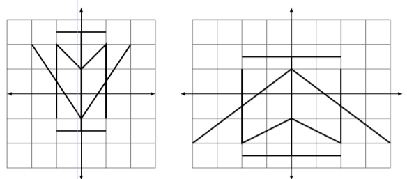
$clipboard_e5e0b2bb8579f849df2d123963ef15990.png$

Figure $\PageIndex{4}$: Transforming the Cartesian plane in Example $\PageIndex{3}$.

A while ago we asked two questions. The first was “How do we find the matrix that performs a given transformation?” We have just answered that question (although we will do more to explore it in the future). The second question was “How does knowing how the unit square is transformed really help us understand how the entire plane is transformed?”

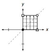
Consider Figure $\PageIndex{5}$ where the unit square (with vertices marked with shapes as before) is shown transformed under an unknown matrix. How does this help us understand how the whole Cartesian plane is transformed? For instance, how can we use this picture to figure out how the point $(2,3)$ will be transformed?

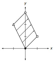
$clipboard_ed369caec0be23384c1b5a441677bd4b2.png$

Figure $\PageIndex{5}$: The unit square under an unknown transformation.

There are two ways to consider the solution to this question. First, we know now how to compute the transformation matrix; the new position of $\vec{e_{1}}$ is the first column of $A$, and the new position of $\vec{e_{2}}$ is the second column of $A$. Therefore, by looking at the figure, we can deduce that $^{6}$

\[A=\left[\begin{array}{cc}{1}&{-1}\\{1}&{2}\end{array}\right]. \nonumber \]

To find where the point $(2,3)$ is sent, simply multiply

\[\left[\begin{array}{cc}{1}&{-1}\\{1}&{2}\end{array}\right]\left[\begin{array}{c}{2}\\{3}\end{array}\right]=\left[\begin{array}{c}{-1}\\{8}\end{array}\right]. \nonumber \]

There is another way of doing this which isn’t as computational – it doesn’t involve computing the transformation matrix. Consider the following equalities:

\[\begin{align}\begin{aligned}\left[\begin{array}{c}{2}\\{3}\end{array}\right]&=\left[\begin{array}{c}{2}\\{0}\end{array}\right]+\left[\begin{array}{c}{0}\\{3}\end{array}\right] \\ &=2\left[\begin{array}{c}{1}\\{0}\end{array}\right] +3\left[\begin{array}{c}{0}\\{1}\end{array}\right] \\ &=2\vec{e_{1}}+3\vec{e_{2}}\end{aligned}\end{align} \nonumber \]

This last equality states something that is somewhat obvious: to arrive at the vector $\left[\begin{array}{c}{2}\\{3}\end{array}\right]$, one needs to go $2$ units in the $\vec{e_{1}}$ direction and $3$ units in the $\vec{e_{2}}$ direction. To find where the point $(2,3)$ is transformed, one needs to go $2$ units in the new $\vec{e_{1}}$ direction and $3$ units in the new $\vec{e_{2}}$ direction. This is demonstrated in Figure $\PageIndex{6}$.

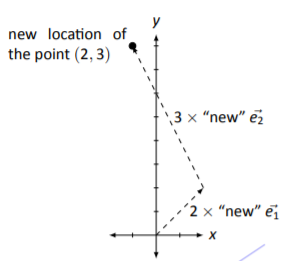
$clipboard_eb692aa98eef5c0a0a87b43e7ca82ee9a.png$

Figure $\PageIndex{6}$: Finding the new location of the point $(2,3)$.

We are coming to grips with how matrix transformations work. We asked two basic questions: “How do we find the matrix for a given transformation?” and “How do we understand the transformation without the matrix?”, and we’ve answered each accompanied by one example. Let’s do another example that demonstrates both techniques at once.

Example $\PageIndex{4}$

First, find the matrix $A$ that transforms the Cartesian plane by stretching it vertically by a factor of $1.5$, then stretches it horizontally by a factor of $0.5$, then rotates it clockwise about the origin $90^{\circ}$. Secondly, using the new locations of $\vec{e_{1}}$ and $\vec{e_{2}}$, find the transformed location of the point $(−1, 2)$.

Solution

To find $A$, first consider the new location of $\vec{e_{1}}$. Stretching the plane vertically does not affect $\vec{e_{1}}$; stretching the plane horizontally by a factor of $0.5$ changes $\vec{e_{1}}$ to $\left[\begin{array}{c}{1/2}\\{0}\end{array}\right]$, and then rotating it $90^\circ$ about the origin moves it to $\left[\begin{array}{c}{0}\\{-1/2}\end{array}\right]$. This is the first column of $A$.

Now consider the new location of $\vec{e_{2}}$. Stretching the plane vertically changes it to $\left[\begin{array}{c}{0}\\{3/2}\end{array}\right]$; stretching horizontally does not affect it, and rotating $90^\circ$ moves it to $\left[\begin{array}{c}{3/2}\\{0}\end{array}\right]$. This is then the second column of $A$. This gives

\[A=\left[\begin{array}{cc}{0}&{3/2}\\{-1/2}&{0}\end{array}\right]. \nonumber \]

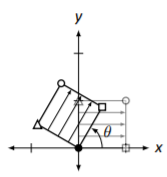
Where does the point $(-1,2)$ get sent to? The corresponding vector $\left[\begin{array}{c}{-1}\\{2}\end{array}\right]$ is found by going $-1$ units in the $\vec{e_{1}}$ direction and $2$ units in the $\vec{e_{2}}$ direction. Therefore, the transformation will send the vector to $-1$ units in the new $\vec{e_{1}}$ direction and $2$ units in the new $\vec{e_{2}}$ direction. This is sketched in Figure $\PageIndex{7}$, along with the transformed unit square. We can also check this multiplicatively:

\[\left[\begin{array}{cc}{0}&{3/2}\\{-1/2}&{0}\end{array}\right]\left[\begin{array}{c}{-1}\\{2}\end{array}\right]=\left[\begin{array}{c}{3}\\{1/2}\end{array}\right]. \nonumber \]

Figure $\PageIndex{8}$ shows the effects of the transformation on another shape.

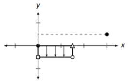
$clipboard_e301aac0f1bc051d646c4502ef742b9e3.png$

Figure $\PageIndex{7}$: Understanding the transformation in Example $\PageIndex{4}$.

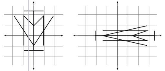
$clipboard_e47c2f051910b3740b023d4c1b6388f2f.png$

Figure $\PageIndex{8}$: Transforming the Cartesian plane in Example $\PageIndex{4}$.

Right now we are focusing on transforming the Cartesian plane – we are making 2D transformations. Knowing how to do this provides a foundation for transforming 3D space,$^{7}$ which, among other things, is very important when producing 3D computer graphics. Basic shapes can be drawn and then rotated, stretched, and/or moved to other regions of space. This also allows for things like “moving the camera view.”

What kinds of transformations are possible? We have already seen some of the things that are possible: rotations, stretches, and flips. We have also mentioned some things that are not possible. For instance, we stated that straight lines always get transformed to straight lines. Therefore, we cannot transform the unit square into a circle using a matrix.

Let’s look at some common transformations of the Cartesian plane and the matrices that perform these operations. In the following figures, a transformation matrix will be given alongside a picture of the transformed unit square. (The original unit square is drawn lightly as well to serve as a reference.)

2D Matrix Transformations

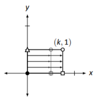
Horizontal stretch by a factor of $k$.

\[\left[\begin{array}{cc}{k}&{0}\\{0}&{1}\end{array}\right]\nonumber \]

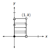
$clipboard_ed9ab4c9ad25a6366ef0d300ab175bf94.png$

Vertical stretch by a factor of $k$.

\[\left[\begin{array}{cc}{1}&{0}\\{0}&{k}\end{array}\right]\nonumber \]

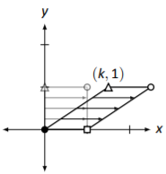
$clipboard_edc6a947e626924b2d0cac3d0ab59f523.png$

Horizontal shear by a factor of $k$.

\[\left[\begin{array}{cc}{1}&{k}\\{0}&{1}\end{array}\right]\nonumber \]

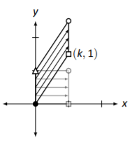
$clipboard_eb6abfdce07bb93f3817f7d412dcf98e5.png$

Vertical shear by a factor of $k$.

\[\left[\begin{array}{cc}{1}&{0}\\{k}&{1}\end{array}\right]\nonumber \]

$clipboard_ef603a700420a3cc4e10a45ec239e3835.png$

Horizontal reflection across the $y$ axis

\[\left[\begin{array}{cc}{-1}&{0}\\{0}&{1}\end{array}\right]\nonumber \]

$clipboard_e7cd824a8abea122d523f2c4c1adc32f2.png$

Vertical reflection across the $x$ axis.

\[\left[\begin{array}{cc}{1}&{0}\\{0}&{-1}\end{array}\right]\nonumber \]

$clipboard_e437a8776f2c2dd42deca9cb391706469.png$

Diagonal reflection across the line $y=x$.

\[\left[\begin{array}{cc}{0}&{1}\\{1}&{0}\end{array}\right]\nonumber \]

$clipboard_e42478112c5b6409e2e67b5d2e0cd37b1.png$

Rotation around the origin by an angle of $\theta$.

\[\left[\begin{array}{cc}{\cos\theta}&{-\sin\theta} \\ {\sin\theta}&{\cos\theta}\end{array}\right]\nonumber \]

$clipboard_e32cae881e4b87cdc2cf1c4a8b563cb0f.png$

Projection onto the $x$ axis.

(Note how the square is "squashed" down onto the $x$-axis.)

\[\left[\begin{array}{cc}{1}&{0}\\{0}&{0}\end{array}\right]\nonumber \]

$clipboard_e230040d2ea452eb7319ff946848d45bd.png$

Projection onto the $y$ axis.

(Note how the square is "squashed" over onto the $y$-axis.)

\[\left[\begin{array}{cc}{0}&{0}\\{0}&{1}\end{array}\right]\nonumber \]

$clipboard_e406f2c30ebb0cf4924a77a2f2ece8fa8.png$

Now that we have seen a healthy list of transformations that we can perform on the Cartesian plane, let’s practice a few more times creating the matrix that gives the desired transformation. In the following example, we develop our understanding one more critical step.

Example $\PageIndex{5}$

Find the matrix $A$ that transforms the Cartesian plane by performing the following operations in order:

Vertical shear by a factor of $0.5$
Counterclockwise roation about the origin by an angle of $\theta=30^{\circ}$
Horizontal stretch by a factor of $2$
Diagonal reflection across the line $y=x$

Solution

Wow! We already know how to do this – sort of. We know we can find the columns of $A$ by tracing where $\vec{e_{1}}$ and $\vec{e_{2}}$ end up, but this also seems difficult. There is so much that is going on. Fortunately, we can accomplish what we need without much difficulty by being systematic.

First, let’s perform the vertical shear. The matrix that performs this is

\[A_{1}=\left[\begin{array}{cc}{1}&{0}\\{0.5}&{1}\end{array}\right]. \nonumber \]

After that, we want to rotate everything clockwise by $30^\circ$. To do this, we use

\[A_{2}=\left[\begin{array}{cc}{\cos 30^{\circ}}&{-\sin 30^{\circ}} \\ {\sin 30^{\circ}}&{\cos 30^{\circ}}\end{array}\right] =\left[\begin{array}{cc}{\sqrt{3}/2}&{-1/2}\\{1/2}&{\sqrt{3}/2}\end{array}\right]. \nonumber \]

In order to do both of these operations, in order, we multiply $A_{2}A_{1}$.$^{8}$

To perform the final two operations, we note that

\[A_{3}=\left[\begin{array}{cc}{2}&{0}\\{0}&{1}\end{array}\right]\quad\text{\and}\quad A_{4}= \left[\begin{array}{cc}{0}&{1}\\{1}&{0}\end{array}\right] \nonumber \]

perform the horizontal stretch and diagonal reflection, respectively. Thus to perform all of the operations “at once,” we need to multiply by

\[\begin{align}\begin{aligned}A&=A_{4}A_{3}A_{2}A_{1} \\ &=\left[\begin{array}{cc}{0}&{1}\\{1}&{0}\end{array}\right]\left[\begin{array}{cc}{2}&{0}\\{0}&{1}\end{array}\right]\left[\begin{array}{cc}{\sqrt{3}/2}&{-1/2} \\ {1/2}&{\sqrt{3}/2}\end{array}\right]\left[\begin{array}{cc}{1}&{0}\\{0.5}&{1}\end{array}\right] \\ &=\left[\begin{array}{cc}{(\sqrt{3}+2)/4}&{\sqrt{3}/2} \\ {(2\sqrt{3}-1)/2}&{-1}\end{array}\right] \\ &\approx\left[\begin{array}{cc}{0.933}&{0.866} \\ {1.232}&{-1}\end{array}\right].\end{aligned}\end{align} \nonumber \]

Let’s consider this closely. Suppose I want to know where a vector $\vec{x}$ ends up. We claim we can find the answer by multiplying $A\vec{x}$. Why does this work? Consider:

\[\begin{align}\begin{aligned}A\vec{x}&=A_{4}A_{3}A_{2}A_{1}\vec{x} \\ &=A_{4}A_{3}A_{2}(A_{1}\vec{x}) &\text{(performs the vertical shear)} \\ &=A_{4}A_{3}(A_{2}\vec{x_{1}}) &\text{(performs the rotation)} \\ &=A_{4}(A_{3}\vec{x_{2}}) &\text{(performs the horizontal stretch)} \\ &=A_{4}\vec{x_{3}} &\text{(performs the diagonal reflection)} \\ &=\vec{x_{4}} &\text{(the result of transforming }\vec{x}\text{)}\end{aligned}\end{align} \nonumber \]

Most readers are not able to visualize exactly what the given list of operations does to the Cartesian plane. In Figure $\PageIndex{9}$ we sketch the transformed unit square; in Figure $\PageIndex{10}$ we sketch a shape and its transformation.

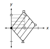
$clipboard_e8b80ae527996806fe9fcaae8bbfa521e.png$

Figure $\PageIndex{9}$: The transformed unit square in Example $\PageIndex{5}$.

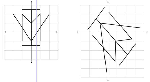
$clipboard_e0e9b602ea6619536720981e170ad2e2e.png$

Figure $\PageIndex{10}$: A transformed shape in Example $\PageIndex{5}$.

Once we know what matrices perform the basic transformations,$^{9}$ performing complex transformations on the Cartesian plane really isn’t that $\ldots$ complex. It boils down to multiplying by a series of matrices.

We’ve shown many examples of transformations that we can do, and we’ve mentioned just a few that we can’t – for instance, we can’t turn a square into a circle. Why not? Why is it that straight lines get sent to straight lines? We spent a lot of time within this text looking at invertible matrices; what connections, if any,$^{10}$ are there between invertible matrices and their transformations on the Cartesian plane?

All these questions require us to think like mathematicians – we are being asked to study the properties of an object we just learned about and their connections to things we’ve already learned. We’ll do all this (and more!) in the following section.

Footnotes

[1] No, we won’t do them one by one.

[2] mathematically, that is called a translation

[3] Although this is less of a surprise, given the result of the previous point.

[4] This observation is a bit more obscure than the first three. It follows from the fact that this corner of the unit square is the “sum” of the other two nonzero corners.

[5] Another way of looking at all of this is to consider what $A\cdot I$ is: of course, it is just $A$. What are the columns of $I$? Just $\vec{e_{1}}$ and $\vec{e_{2}}$.

[6] At least, $A$ is close to that. The square corner could actually be at the point $(1.01, .99)$.

[7] Actually, it provides a foundation for doing it in 4D, 5D, $\ldots$, 17D, etc. Those are just harder to visualize.

[8] The reader might ask, “Is it important to do multiply these in that order? Could we have multiplied $A_{1}A_{2}$ instead?” Our answer starts with “Is matrix multiplication commutative?” The answer to our question is “No,” so the answers to the reader’s questions are “Yes” and “No,” respectively.

[9] or know where to find them

[10] By now, the reader should expect connections to exist.

Search

Example \(\PageIndex{5}\)

Learning Objectives

Example \(\PageIndex{1}\)

Example \(\PageIndex{2}\)

Example \(\PageIndex{3}\)

Example \(\PageIndex{4}\)

2D Matrix Transformations

Example \(\PageIndex{5}\)

Footnotes