2.1: Vectors
- Page ID
- 70186

\( \newcommand{\vecs}[1]{\overset { \scriptstyle \rightharpoonup} {\mathbf{#1}} } \)
\( \newcommand{\vecd}[1]{\overset{-\!-\!\rightharpoonup}{\vphantom{a}\smash {#1}}} \)
\( \newcommand{\dsum}{\displaystyle\sum\limits} \)
\( \newcommand{\dint}{\displaystyle\int\limits} \)
\( \newcommand{\dlim}{\displaystyle\lim\limits} \)
\( \newcommand{\id}{\mathrm{id}}\) \( \newcommand{\Span}{\mathrm{span}}\)
( \newcommand{\kernel}{\mathrm{null}\,}\) \( \newcommand{\range}{\mathrm{range}\,}\)
\( \newcommand{\RealPart}{\mathrm{Re}}\) \( \newcommand{\ImaginaryPart}{\mathrm{Im}}\)
\( \newcommand{\Argument}{\mathrm{Arg}}\) \( \newcommand{\norm}[1]{\| #1 \|}\)
\( \newcommand{\inner}[2]{\langle #1, #2 \rangle}\)
\( \newcommand{\Span}{\mathrm{span}}\)
\( \newcommand{\id}{\mathrm{id}}\)
\( \newcommand{\Span}{\mathrm{span}}\)
\( \newcommand{\kernel}{\mathrm{null}\,}\)
\( \newcommand{\range}{\mathrm{range}\,}\)
\( \newcommand{\RealPart}{\mathrm{Re}}\)
\( \newcommand{\ImaginaryPart}{\mathrm{Im}}\)
\( \newcommand{\Argument}{\mathrm{Arg}}\)
\( \newcommand{\norm}[1]{\| #1 \|}\)
\( \newcommand{\inner}[2]{\langle #1, #2 \rangle}\)
\( \newcommand{\Span}{\mathrm{span}}\) \( \newcommand{\AA}{\unicode[.8,0]{x212B}}\)
\( \newcommand{\vectorA}[1]{\vec{#1}} % arrow\)
\( \newcommand{\vectorAt}[1]{\vec{\text{#1}}} % arrow\)
\( \newcommand{\vectorB}[1]{\overset { \scriptstyle \rightharpoonup} {\mathbf{#1}} } \)
\( \newcommand{\vectorC}[1]{\textbf{#1}} \)
\( \newcommand{\vectorD}[1]{\overrightarrow{#1}} \)
\( \newcommand{\vectorDt}[1]{\overrightarrow{\text{#1}}} \)
\( \newcommand{\vectE}[1]{\overset{-\!-\!\rightharpoonup}{\vphantom{a}\smash{\mathbf {#1}}}} \)
\( \newcommand{\vecs}[1]{\overset { \scriptstyle \rightharpoonup} {\mathbf{#1}} } \)
\(\newcommand{\longvect}{\overrightarrow}\)
\( \newcommand{\vecd}[1]{\overset{-\!-\!\rightharpoonup}{\vphantom{a}\smash {#1}}} \)
\(\newcommand{\avec}{\mathbf a}\) \(\newcommand{\bvec}{\mathbf b}\) \(\newcommand{\cvec}{\mathbf c}\) \(\newcommand{\dvec}{\mathbf d}\) \(\newcommand{\dtil}{\widetilde{\mathbf d}}\) \(\newcommand{\evec}{\mathbf e}\) \(\newcommand{\fvec}{\mathbf f}\) \(\newcommand{\nvec}{\mathbf n}\) \(\newcommand{\pvec}{\mathbf p}\) \(\newcommand{\qvec}{\mathbf q}\) \(\newcommand{\svec}{\mathbf s}\) \(\newcommand{\tvec}{\mathbf t}\) \(\newcommand{\uvec}{\mathbf u}\) \(\newcommand{\vvec}{\mathbf v}\) \(\newcommand{\wvec}{\mathbf w}\) \(\newcommand{\xvec}{\mathbf x}\) \(\newcommand{\yvec}{\mathbf y}\) \(\newcommand{\zvec}{\mathbf z}\) \(\newcommand{\rvec}{\mathbf r}\) \(\newcommand{\mvec}{\mathbf m}\) \(\newcommand{\zerovec}{\mathbf 0}\) \(\newcommand{\onevec}{\mathbf 1}\) \(\newcommand{\real}{\mathbb R}\) \(\newcommand{\twovec}[2]{\left[\begin{array}{r}#1 \\ #2 \end{array}\right]}\) \(\newcommand{\ctwovec}[2]{\left[\begin{array}{c}#1 \\ #2 \end{array}\right]}\) \(\newcommand{\threevec}[3]{\left[\begin{array}{r}#1 \\ #2 \\ #3 \end{array}\right]}\) \(\newcommand{\cthreevec}[3]{\left[\begin{array}{c}#1 \\ #2 \\ #3 \end{array}\right]}\) \(\newcommand{\fourvec}[4]{\left[\begin{array}{r}#1 \\ #2 \\ #3 \\ #4 \end{array}\right]}\) \(\newcommand{\cfourvec}[4]{\left[\begin{array}{c}#1 \\ #2 \\ #3 \\ #4 \end{array}\right]}\) \(\newcommand{\fivevec}[5]{\left[\begin{array}{r}#1 \\ #2 \\ #3 \\ #4 \\ #5 \\ \end{array}\right]}\) \(\newcommand{\cfivevec}[5]{\left[\begin{array}{c}#1 \\ #2 \\ #3 \\ #4 \\ #5 \\ \end{array}\right]}\) \(\newcommand{\mattwo}[4]{\left[\begin{array}{rr}#1 \amp #2 \\ #3 \amp #4 \\ \end{array}\right]}\) \(\newcommand{\laspan}[1]{\text{Span}\{#1\}}\) \(\newcommand{\bcal}{\cal B}\) \(\newcommand{\ccal}{\cal C}\) \(\newcommand{\scal}{\cal S}\) \(\newcommand{\wcal}{\cal W}\) \(\newcommand{\ecal}{\cal E}\) \(\newcommand{\coords}[2]{\left\{#1\right\}_{#2}}\) \(\newcommand{\gray}[1]{\color{gray}{#1}}\) \(\newcommand{\lgray}[1]{\color{lightgray}{#1}}\) \(\newcommand{\rank}{\operatorname{rank}}\) \(\newcommand{\row}{\text{Row}}\) \(\newcommand{\col}{\text{Col}}\) \(\renewcommand{\row}{\text{Row}}\) \(\newcommand{\nul}{\text{Nul}}\) \(\newcommand{\var}{\text{Var}}\) \(\newcommand{\corr}{\text{corr}}\) \(\newcommand{\len}[1]{\left|#1\right|}\) \(\newcommand{\bbar}{\overline{\bvec}}\) \(\newcommand{\bhat}{\widehat{\bvec}}\) \(\newcommand{\bperp}{\bvec^\perp}\) \(\newcommand{\xhat}{\widehat{\xvec}}\) \(\newcommand{\vhat}{\widehat{\vvec}}\) \(\newcommand{\uhat}{\widehat{\uvec}}\) \(\newcommand{\what}{\widehat{\wvec}}\) \(\newcommand{\Sighat}{\widehat{\Sigma}}\) \(\newcommand{\lt}{<}\) \(\newcommand{\gt}{>}\) \(\newcommand{\amp}{&}\) \(\definecolor{fillinmathshade}{gray}{0.9}\)- Learn how to add and scale vectors in \(\mathbb{R}^n\text{,}\) both algebraically and geometrically.
- Understand linear combinations geometrically.
- Pictures: vector addition, vector subtraction, linear combinations.
- Vocabulary words: vector, linear combination.
Vectors in \(\mathbb{R}^n\)
We have been drawing points in \(\mathbb{R}^n\) as dots in the line, plane, space, etc. We can also draw them as arrows. Since we have two geometric interpretations in mind, we now discuss the relationship between the two points of view.
Again, a point in \(\mathbb{R}^n\) is drawn as a dot.
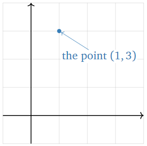
Figure \(\PageIndex{1}\)
A vector is a point in \(\mathbb{R}^n\text{,}\) drawn as an arrow.
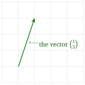
Figure \(\PageIndex{2}\)
The difference is purely psychological: points and vectors are both just lists of numbers.
When we think of a point in \(\mathbb{R}^n\) as a vector, we will usually write it vertically, like a matrix with one column:
\[v=\left(\begin{array}{c}1\\3\end{array}\right).\nonumber\]
We will also write \(0\) for the zero vector.
Why make the distinction between points and vectors? A vector need not start at the origin: it can be located anywhere! In other words, an arrow is determined by its length and its direction, not by its location. For instance, these arrows all represent the vector \(\color{green}{\left(\begin{array}{c}1\\2\end{array}\right)}\).
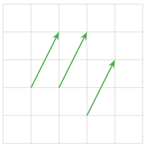
Figure \(\PageIndex{4}\)
Unless otherwise specified, we will assume that all vectors start at the origin.
Vectors makes sense in the real world: many physical quantities, such as velocity, are represented as vectors. But it makes more sense to think of the velocity of a car as being located at the car.
Some authors use boldface letters to represent vectors, as in “\(\mathbf v\)”, or use arrows, as in “\(\vec v\)”. As it is usually clear from context if a letter represents a vector, we do not decorate vectors in this way.
Another way to think about a vector is as a difference between two points, or the arrow from one point to another. For instance, \({1\choose 2}\) is the arrow from \((1,1)\) to \((2,3)\).
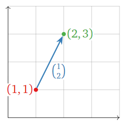
Figure \(\PageIndex{5}\)
Vector Algebra and Geometry
Here we learn how to add vectors together and how to multiply vectors by numbers, both algebraically and geometrically.
- We can add two vectors together:
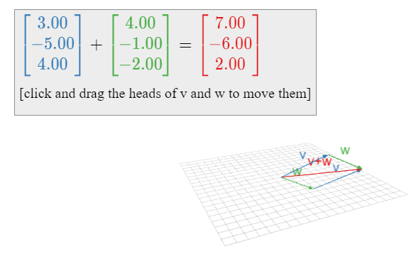
\[\left(\begin{array}{c}a\\b\\c\end{array}\right) +\left(\begin{array}{c}x\\y\\z\end{array}\right)=\left(\begin{array}{c}a+x \\ b+y\\c+z\end{array}\right).\nonumber\] - We can multiply, or scale, a vector by a real number \(c\text{:}\)
\[\color{red}{c}\color{black}{\left(\begin{array}{c}x\\y\\z\end{array}\right)} =\left(\begin{array}{c}\color{red}{c}\color{black}{\:\cdot\: x} \\ \color{red}{c}\color{black}{\:\cdot\: y}\\ \color{red}{c}\color{black}{\:\cdot\: z}\end{array}\right).\nonumber\]
We call \(c\) a scalar to distinguish it from a vector. If \(v\) is a vector and \(c\) is a scalar, then \(cv\) is called a scalar multiple of \(v\).
Addition and scalar multiplication work in the same way for vectors of length \(n\).
\[\left(\begin{array}{c}1\\2\\3\end{array}\right) +\left(\begin{array}{c}4\\5\\6\end{array}\right)=\left(\begin{array}{c}5\\7\\9\end{array}\right)\quad\text{and}\quad -2\left(\begin{array}{c}1\\2\\3\end{array}\right)=\left(\begin{array}{c}-2\\-4\\-6\end{array}\right).\nonumber\]
The Parallelogram Law for Vector Addition
Geometrically, the sum of two vectors \(v,w\) is obtained as follows: place the tail of \(w\) at the head of \(v\). Then \(v+w\) is the vector whose tail is the tail of \(v\) and whose head is the head of \(w\). Doing this both ways creates a parallelogram. For example,
\[\color{blue}{\left(\begin{array}{c}1\\3\end{array}\right)}\color{black}{+}\color{green}{\left(\begin{array}{c}4\\2\end{array}\right)}\color{black}{=\left(\begin{array}{c}5\\5\end{array}\right).}\nonumber\]
Why? The width of \(v+w\) is the sum of the widths, and likewise with the heights.
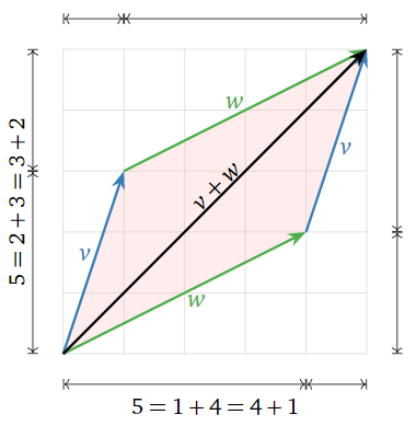
Figure \(\PageIndex{6}\)
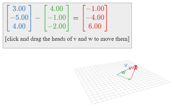
Vector Subtraction
Geometrically, the difference of two vectors \(v,w\) is obtained as follows: place the tail of \(v\) and \(w\) at the same point. Then \(v-w\) is the vector from the head of \(w\) to the head of \(v\). For example,
\[\color{blue}{\left(\begin{array}{c}1\\4\end{array}\right)}\color{black}{-}\color{green}{\left(\begin{array}{c}4\\2\end{array}\right)}\color{black}{=\left(\begin{array}{c}-3\\2\end{array}\right).}\nonumber\]
Why? If you add \(v-w\) to \(w\text{,}\) you get \(v\).
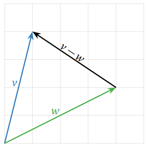
Figure \(\PageIndex{8}\)
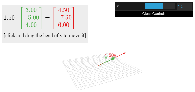
Scalar Multiplication
A scalar multiple of a vector \(v\) has the same (or opposite) direction, but a different length. For instance, \(2v\) is the vector in the direction of \(v\) but twice as long, and \(-\frac 12v\) is the vector in the opposite direction of \(v\text{,}\) but half as long. Note that the set of all scalar multiples of a (nonzero) vector \(v\) is a line.
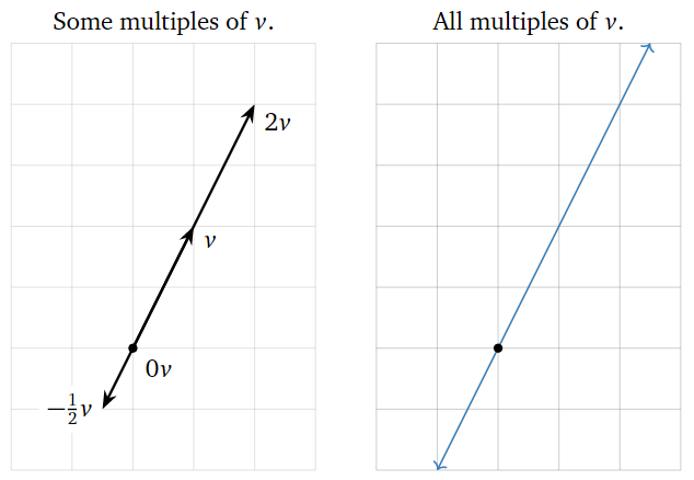
Figure \(\PageIndex{10}\)
Linear Combinations
We can add and scale vectors in the same equation.
Let \(c_1,c_2,\ldots,c_k\) be scalars, and let \(v_1,v_2,\ldots,v_k\) be vectors in \(\mathbb{R}^n\). The vector in \(\mathbb{R}^n\)
\[ c_1v_1 + c_2v_2 + \cdots + c_kv_k \nonumber \]
is called a linear combination of the vectors \(v_1,v_2,\ldots,v_k\text{,}\) with weights or coefficients \(c_1,c_2,\ldots,c_k\).
Geometrically, a linear combination is obtained by stretching / shrinking the vectors \(v_1,v_2,\ldots,v_k\) according to the coefficients, then adding them together using the parallelogram law.
Let \(v_1 = {1\choose 2}\) and \(v_2 = {1\choose 0}\). Here are some linear combinations of \(v_1\) and \(v_2\text{,}\) drawn as points.
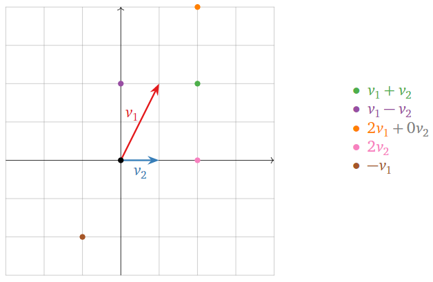
Figure \(\PageIndex{12}\)
The locations of these points are found using the parallelogram law for vector addition. Any vector on the plane is a linear combination of \(v_1\) and \(v_2\text{,}\) with suitable coefficients.
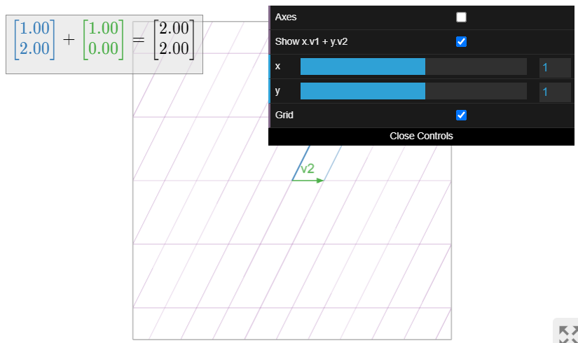
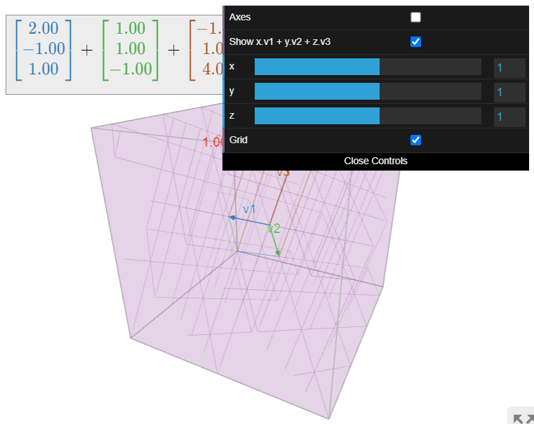
Figure \(\PageIndex{13}\): Linear combinations of two vectors in \(\mathbb{R}^2\text{:}\) move the sliders to change the coefficients of \(v_1\) and \(v_2\). Note that any vector on the plane can be obtained as a linear combination of \(v_1,v_2\) with suitable coefficients.
A linear combination of a single vector \(v = {1\choose 2}\) is just a scalar multiple of \(v\). So some examples include
\[v=\left(\begin{array}{c}1\\2\end{array}\right),\quad \frac{3}{2}v=\left(\begin{array}{c}3/2\\3\end{array}\right),\quad -\frac{1}{2}v=\left(\begin{array}{c}-1/2\\-1\end{array}\right),\quad\cdots\nonumber\]
The set of all linear combinations is the line through \(v\). (Unless \(v=0\text{,}\) in which case any scalar multiple of \(v\) is again \(0\).)
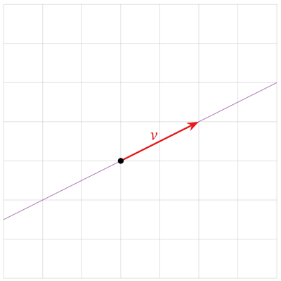
Figure \(\PageIndex{15}\)
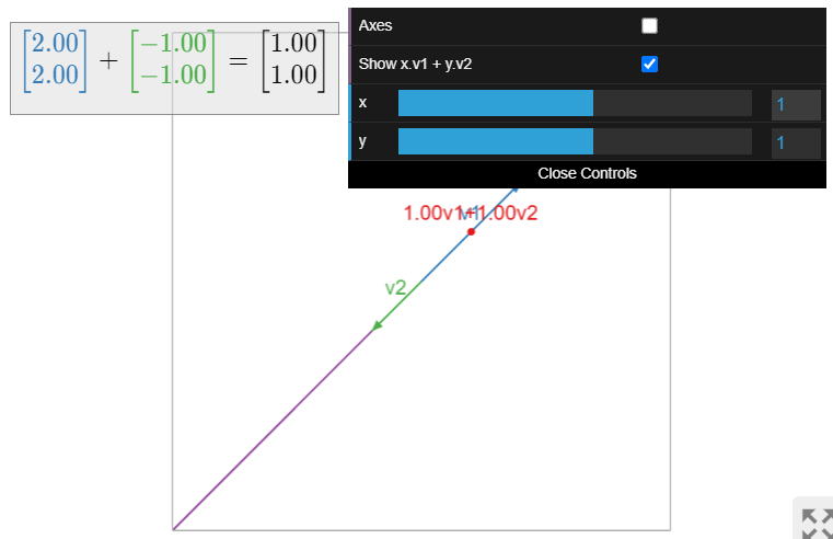
The set of all linear combinations of the vectors
\[v_{1}=\left(\begin{array}{c}2\\2\end{array}\right)\quad\text{and}\quad v_{2}=\left(\begin{array}{c}-1\\-1\end{array}\right)\nonumber\]
is the line containing both vectors.
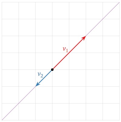
Figure \(\PageIndex{16}\)
The difference between this and Example \(\PageIndex{6}\) is that both vectors lie on the same line. Hence any scalar multiples of \(v_1,v_2\) lie on that line, as does their sum.