2.2: Vector Equations and Spans
- Page ID
- 70187
\( \newcommand{\vecs}[1]{\overset { \scriptstyle \rightharpoonup} {\mathbf{#1}} } \)
\( \newcommand{\vecd}[1]{\overset{-\!-\!\rightharpoonup}{\vphantom{a}\smash {#1}}} \)
\( \newcommand{\dsum}{\displaystyle\sum\limits} \)
\( \newcommand{\dint}{\displaystyle\int\limits} \)
\( \newcommand{\dlim}{\displaystyle\lim\limits} \)
\( \newcommand{\id}{\mathrm{id}}\) \( \newcommand{\Span}{\mathrm{span}}\)
( \newcommand{\kernel}{\mathrm{null}\,}\) \( \newcommand{\range}{\mathrm{range}\,}\)
\( \newcommand{\RealPart}{\mathrm{Re}}\) \( \newcommand{\ImaginaryPart}{\mathrm{Im}}\)
\( \newcommand{\Argument}{\mathrm{Arg}}\) \( \newcommand{\norm}[1]{\| #1 \|}\)
\( \newcommand{\inner}[2]{\langle #1, #2 \rangle}\)
\( \newcommand{\Span}{\mathrm{span}}\)
\( \newcommand{\id}{\mathrm{id}}\)
\( \newcommand{\Span}{\mathrm{span}}\)
\( \newcommand{\kernel}{\mathrm{null}\,}\)
\( \newcommand{\range}{\mathrm{range}\,}\)
\( \newcommand{\RealPart}{\mathrm{Re}}\)
\( \newcommand{\ImaginaryPart}{\mathrm{Im}}\)
\( \newcommand{\Argument}{\mathrm{Arg}}\)
\( \newcommand{\norm}[1]{\| #1 \|}\)
\( \newcommand{\inner}[2]{\langle #1, #2 \rangle}\)
\( \newcommand{\Span}{\mathrm{span}}\) \( \newcommand{\AA}{\unicode[.8,0]{x212B}}\)
\( \newcommand{\vectorA}[1]{\vec{#1}} % arrow\)
\( \newcommand{\vectorAt}[1]{\vec{\text{#1}}} % arrow\)
\( \newcommand{\vectorB}[1]{\overset { \scriptstyle \rightharpoonup} {\mathbf{#1}} } \)
\( \newcommand{\vectorC}[1]{\textbf{#1}} \)
\( \newcommand{\vectorD}[1]{\overrightarrow{#1}} \)
\( \newcommand{\vectorDt}[1]{\overrightarrow{\text{#1}}} \)
\( \newcommand{\vectE}[1]{\overset{-\!-\!\rightharpoonup}{\vphantom{a}\smash{\mathbf {#1}}}} \)
\( \newcommand{\vecs}[1]{\overset { \scriptstyle \rightharpoonup} {\mathbf{#1}} } \)
\(\newcommand{\longvect}{\overrightarrow}\)
\( \newcommand{\vecd}[1]{\overset{-\!-\!\rightharpoonup}{\vphantom{a}\smash {#1}}} \)
\(\newcommand{\avec}{\mathbf a}\) \(\newcommand{\bvec}{\mathbf b}\) \(\newcommand{\cvec}{\mathbf c}\) \(\newcommand{\dvec}{\mathbf d}\) \(\newcommand{\dtil}{\widetilde{\mathbf d}}\) \(\newcommand{\evec}{\mathbf e}\) \(\newcommand{\fvec}{\mathbf f}\) \(\newcommand{\nvec}{\mathbf n}\) \(\newcommand{\pvec}{\mathbf p}\) \(\newcommand{\qvec}{\mathbf q}\) \(\newcommand{\svec}{\mathbf s}\) \(\newcommand{\tvec}{\mathbf t}\) \(\newcommand{\uvec}{\mathbf u}\) \(\newcommand{\vvec}{\mathbf v}\) \(\newcommand{\wvec}{\mathbf w}\) \(\newcommand{\xvec}{\mathbf x}\) \(\newcommand{\yvec}{\mathbf y}\) \(\newcommand{\zvec}{\mathbf z}\) \(\newcommand{\rvec}{\mathbf r}\) \(\newcommand{\mvec}{\mathbf m}\) \(\newcommand{\zerovec}{\mathbf 0}\) \(\newcommand{\onevec}{\mathbf 1}\) \(\newcommand{\real}{\mathbb R}\) \(\newcommand{\twovec}[2]{\left[\begin{array}{r}#1 \\ #2 \end{array}\right]}\) \(\newcommand{\ctwovec}[2]{\left[\begin{array}{c}#1 \\ #2 \end{array}\right]}\) \(\newcommand{\threevec}[3]{\left[\begin{array}{r}#1 \\ #2 \\ #3 \end{array}\right]}\) \(\newcommand{\cthreevec}[3]{\left[\begin{array}{c}#1 \\ #2 \\ #3 \end{array}\right]}\) \(\newcommand{\fourvec}[4]{\left[\begin{array}{r}#1 \\ #2 \\ #3 \\ #4 \end{array}\right]}\) \(\newcommand{\cfourvec}[4]{\left[\begin{array}{c}#1 \\ #2 \\ #3 \\ #4 \end{array}\right]}\) \(\newcommand{\fivevec}[5]{\left[\begin{array}{r}#1 \\ #2 \\ #3 \\ #4 \\ #5 \\ \end{array}\right]}\) \(\newcommand{\cfivevec}[5]{\left[\begin{array}{c}#1 \\ #2 \\ #3 \\ #4 \\ #5 \\ \end{array}\right]}\) \(\newcommand{\mattwo}[4]{\left[\begin{array}{rr}#1 \amp #2 \\ #3 \amp #4 \\ \end{array}\right]}\) \(\newcommand{\laspan}[1]{\text{Span}\{#1\}}\) \(\newcommand{\bcal}{\cal B}\) \(\newcommand{\ccal}{\cal C}\) \(\newcommand{\scal}{\cal S}\) \(\newcommand{\wcal}{\cal W}\) \(\newcommand{\ecal}{\cal E}\) \(\newcommand{\coords}[2]{\left\{#1\right\}_{#2}}\) \(\newcommand{\gray}[1]{\color{gray}{#1}}\) \(\newcommand{\lgray}[1]{\color{lightgray}{#1}}\) \(\newcommand{\rank}{\operatorname{rank}}\) \(\newcommand{\row}{\text{Row}}\) \(\newcommand{\col}{\text{Col}}\) \(\renewcommand{\row}{\text{Row}}\) \(\newcommand{\nul}{\text{Nul}}\) \(\newcommand{\var}{\text{Var}}\) \(\newcommand{\corr}{\text{corr}}\) \(\newcommand{\len}[1]{\left|#1\right|}\) \(\newcommand{\bbar}{\overline{\bvec}}\) \(\newcommand{\bhat}{\widehat{\bvec}}\) \(\newcommand{\bperp}{\bvec^\perp}\) \(\newcommand{\xhat}{\widehat{\xvec}}\) \(\newcommand{\vhat}{\widehat{\vvec}}\) \(\newcommand{\uhat}{\widehat{\uvec}}\) \(\newcommand{\what}{\widehat{\wvec}}\) \(\newcommand{\Sighat}{\widehat{\Sigma}}\) \(\newcommand{\lt}{<}\) \(\newcommand{\gt}{>}\) \(\newcommand{\amp}{&}\) \(\definecolor{fillinmathshade}{gray}{0.9}\)- Understand the equivalence between a system of linear equations and a vector equation.
- Learn the definition of \(\text{Span}\{x_1,x_2,\ldots,x_k\}\text{,}\) and how to draw pictures of spans.
- Recipe: solve a vector equation using augmented matrices / decide if a vector is in a span.
- Pictures: an inconsistent system of equations, a consistent system of equations, spans in \(\mathbb{R}^2\) and \(\mathbb{R}^3\).
- Vocabulary word: vector equation.
- Essential vocabulary word: span.
Vector Equations
An equation involving vectors with \(n\) coordinates is the same as \(n\) equations involving only numbers. For example, the equation
\[x\left(\begin{array}{c}1\\2\\6\end{array}\right) +y\left(\begin{array}{c}-1\\-2\\-1\end{array}\right)=\left(\begin{array}{c}8\\16\\3\end{array}\right)\nonumber\]
simplifies to
\[\left(\begin{array}{c}x\\2x\\6x\end{array}\right)+\left(\begin{array}{c}-y\\-2y\\-y\end{array}\right)=\left(\begin{array}{c}8\\16\\3\end{array}\right)\quad\text{or}\quad\left(\begin{array}{c}x-y\\2x-2y\\6x-y\end{array}\right)=\left(\begin{array}{c}8\\16\\3\end{array}\right).\nonumber\]
For two vectors to be equal, all of their coordinates must be equal, so this is just the system of linear equations
\[\left\{\begin{array}{rrrrc}x &-& y &=& 8\\ 2x &-& 2y &=& 16\\ 6x &-& y &=& 3.\end{array}\right.\nonumber\]
A vector equation is an equation involving a linear combination of vectors with possibly unknown coefficients.
Asking whether or not a vector equation has a solution is the same as asking if a given vector is a linear combination of some other given vectors.
For example the vector equation above is asking if the vector \((8,16,3)\) is a linear combination of the vectors \((1,2,6)\) and \((-1,2,-1)\).
The thing we really care about is solving systems of linear equations, not solving vector equations. The whole point of vector equations is that they give us a different, and more geometric, way of viewing systems of linear equations.
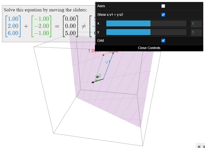
Below we will show that the above system of equations is consistent. Equivalently, this means that the above vector equation has a solution. In other words, there is a linear combination of \((1,2,6)\) and \((-1,2,-1)\) that equals \((8,16,3)\). We can visualize the last statement geometrically. Therefore, the following Figure \(\PageIndex{1}\) gives a picture of a consistent system of equations. Compare with Figure \(\PageIndex{2}\), which shows a picture of an inconsistent system.
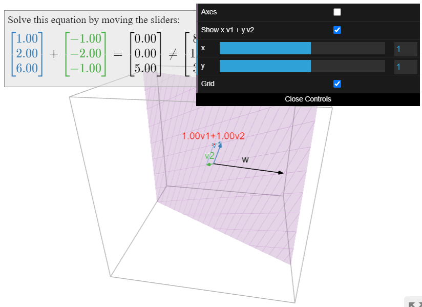
In order to actually solve the vector equation
\[x\color{Red}{\left(\begin{array}{c}1\\2\\6\end{array}\right)} \color{black}{+y}\color{Green}{\left(\begin{array}{c}-1\\-2\\-1\end{array}\right)}\color{black}{=}\color{blue}{\left(\begin{array}{c}8\\16\\3\end{array}\right)}\color{black}{,}\nonumber\]
one has to solve the system of linear equations
\[\left\{\begin{array}{rrrrc} x &-& y &=& 8\\ 2x &-& 2y &=& 16\\ 6x &-& y &=& 3.\end{array}\right. \nonumber\]
This means forming the augmented matrix
\[\left(\begin{array}{cc|c}\color{Red}{1}&\color{Green}{-1}&\color{blue}{8} \\ \color{Red}{2}&\color{Green}{-2}&\color{blue}{16}\\ \color{Red}{6}&\color{Green}{-1} &\color{blue}{3}\end{array}\right)\nonumber\]
and row reducing. Note that the columns of the augmented matrix are the vectors from the original vector equation, so it is not actually necessary to write the system of equations: one can go directly from the vector equation to the augmented matrix by “smooshing the vectors together”. In Example \(\PageIndex{1}\) we carry out the row reduction and find the solution.
Is \(\left(\begin{array}{c}8\\16\\3\end{array}\right)\) a linear combination of \(\left(\begin{array}{c}1\\2\\6\end{array}\right)\) and \(\left(\begin{array}{c}-1\\-2\\-1\end{array}\right)\)?
Solution
As discussed above, this question boils down to a row reduction:
\[\left(\begin{array}{cc|c} 1&-1&8 \\ 2&-2&16 \\ 6&-1&3\end{array}\right) \quad\xrightarrow{\text{RREF}}\quad \left(\begin{array}{cc|c} 1&0&-1 \\ 0&1&-9 \\ 0&0&0\end{array}\right).\nonumber\]
From this we see that the equation is consistent, and the solution is \(x=-1\) and \(y=-9\). We conclude that \(\left(\begin{array}{c}8\\16\\3\end{array}\right)\) is indeed a linear combination of \(\left(\begin{array}{c}1\\2\\6\end{array}\right)\) and \(\left(\begin{array}{c}-1\\-2\\-1\end{array}\right)\), with coefficients \(-1\) and \(-9\text{:}\)
\[-\left(\begin{array}{c}1\\2\\6\end{array}\right)-9\left(\begin{array}{c}-1\\-2\\-1\end{array}\right)=\left(\begin{array}{c}8\\6\\3\end{array}\right).\nonumber\]
In general, the vector equation
\[ x_1v_1 + x_2v_2 + \cdots + x_kv_k = b \nonumber \]
where \(v_1,v_2,\ldots,v_k,\,b\) are vectors in \(\mathbb{R}^n\) and \(x_1,x_2,\ldots,x_k\) are unknown scalars, has the same solution set as the linear system with augmented matrix
\[\left(\begin{array}{cccc|c} | & |&\quad &|&| \\ v_1 &v_2 &\cdots &v_k &b \\ |&|&\quad &|&|\end{array}\right)\nonumber\]
whose columns are the \(v_i\)’s and the \(b\)’s.
Now we have three equivalent ways of thinking about a linear system:
- As a system of equations:
\[\left\{\begin{array}{rrrrrrr} 2x_1 &+& 3x_2 &-& 2x_3 &=& 7\\ x_1 &-& x_2 &-& 3x_3 &=& 5\end{array}\right.\nonumber\] - As an augmented matrix:
\[\left(\begin{array}{ccc|c} 2&3&-2&7 \\ 1&-1&-3&5\end{array}\right)\nonumber\] - As a vector equation (\(x_1v_1 + x_2v_2 + \cdots + x_nv_n = b\)):
\[x_{1}\left(\begin{array}{c}2\\1\end{array}\right)+x_{2}\left(\begin{array}{c}3\\-1\end{array}\right)+x_{3}\left(\begin{array}{c}-2\\-3\end{array}\right)=\left(\begin{array}{c}7\\5\end{array}\right)\nonumber\]
The third is geometric in nature: it lends itself to drawing pictures.
Spans
It will be important to know what are all linear combinations of a set of vectors \(v_1,v_2,\ldots,v_k\) in \(\mathbb{R}^n\). In other words, we would like to understand the set of all vectors \(b\) in \(\mathbb{R}^n\) such that the vector equation (in the unknowns \(x_1,x_2,\ldots,x_k\))
\[ x_1v_1 + x_2v_2 + \cdots + x_kv_k = b \nonumber \]
has a solution (i.e. is consistent).
Let \(v_1,v_2,\ldots,v_k\) be vectors in \(\mathbb{R}^n\). The span of \(v_1,v_2,\ldots,v_k\) is the collection of all linear combinations of \(v_1,v_2,\ldots,v_k\text{,}\) and is denoted \(\text{Span}\{v_1,v_2,\ldots,v_k\}\). In symbols:
\[ \text{Span}\{v_1,v_2,\ldots,v_k\} = \bigl\{x_1v_1 + x_2v_2 + \cdots + x_kv_k \mid x_1,x_2,\ldots,x_k \text{ in }\mathbb{R}\bigr\} \nonumber \]
We also say that \(\text{Span}\{v_1,v_2,\ldots,v_k\}\) is the subset spanned by or generated by the vectors \(v_1,v_2,\ldots,v_k\).
The above definition, Definition \(\PageIndex{2}\) is the first of several essential definitions that we will see in this textbook. They are essential in that they form the essence of the subject of linear algebra: learning linear algebra means (in part) learning these definitions. All of the definitions are important, but it is essential that you learn and understand the definitions marked as such.
The notation
\[ \bigl\{x_1v_1 + x_2v_2 + \cdots + x_kv_k \mid x_1,x_2,\ldots,x_k \text{ in }\mathbb{R}\bigr\} \nonumber \]
reads as: “the set of all things of the form \(x_1v_1 + x_2v_2 + \cdots + x_kv_k\) such that \(x_1,x_2,\ldots,x_k\) are in \(\mathbb{R}\).” The vertical line is “such that”; everything to the left of it is “the set of all things of this form”, and everything to the right is the condition that those things must satisfy to be in the set. Specifying a set in this way is called set builder notation.
All mathematical notation is only shorthand: any sequence of symbols must translate into a usual sentence.
Now we have three equivalent ways of making the same statement:
- A vector \(b\) is in the span of \(v_1,v_2,\ldots,v_k\).
- The vector equation
\[x_1 v_1 +x_2 v_2 +\cdots +x_k v_k =b\nonumber\]
has a solution. - The linear system with augmented matrix
\[\left(\begin{array}{cccc|c} |&|&\quad &|&| \\ v_1 &v_2 &\cdots &v_k &b \\ |&|&\quad &|&| \end{array}\right)\nonumber\]
is consistent.
Equivalent means that, for any given list of vectors \(v_1,v_2,\ldots,v_k,\,b\text{,}\) either all three statements are true, or all three statements are false.
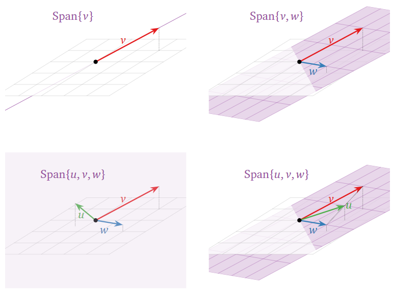
Pictures of Spans.
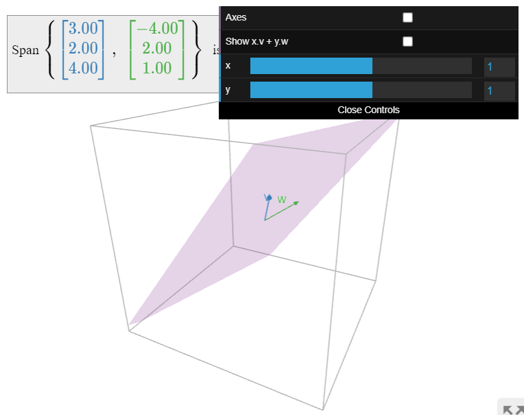
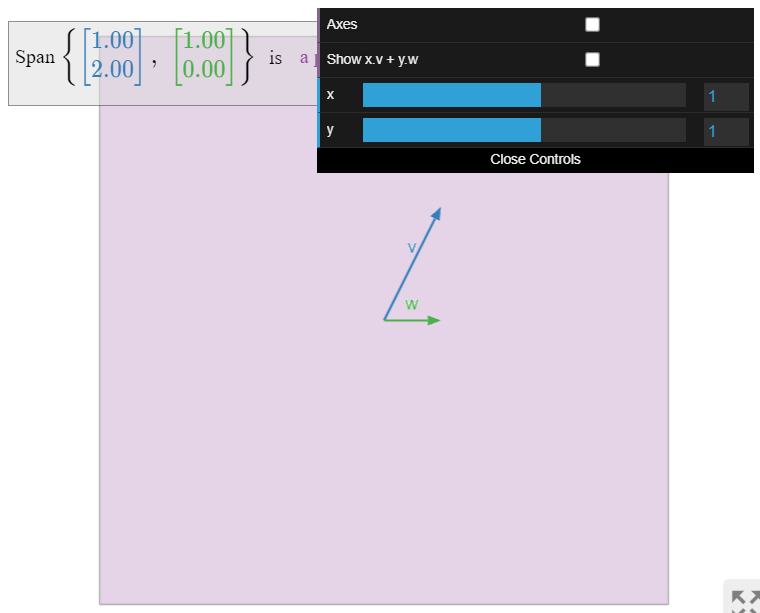
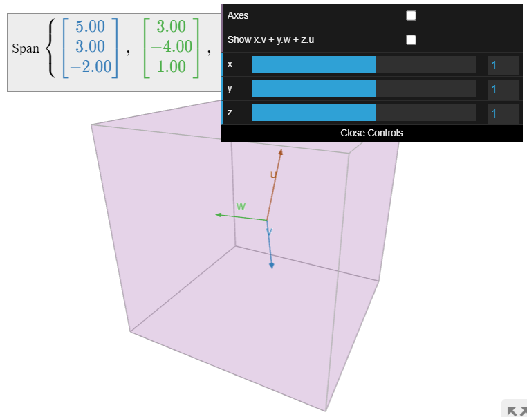
Drawing a picture of \(\text{Span}\{v_1,v_2,\ldots,v_k\}\) is the same as drawing a picture of all linear combinations of \(v_1,v_2,\ldots,v_k\).
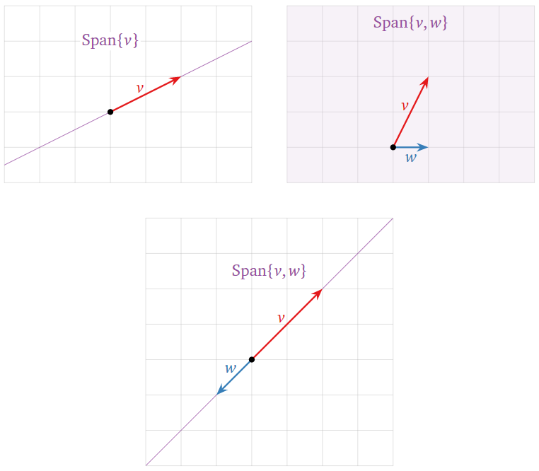
Figure \(\PageIndex{3}\): Pictures of spans in \(\mathbb{R}^2\).
