
2.3: Matrix Equations
- Page ID
- 70188

- Understand the equivalence between a system of linear equations, an augmented matrix, a vector equation, and a matrix equation.
- Characterize the vectors \(b\) such that \(Ax=b\) is consistent, in terms of the span of the columns of \(A\).
- Characterize matrices \(A\) such that \(Ax=b\) is consistent for all vectors \(b\).
- Recipe: multiply a vector by a matrix (two ways).
- Picture: the set of all vectors \(b\) such that \(Ax=b\) is consistent.
- Vocabulary word: matrix equation.
The Matrix Equation \(Ax=b\)
In this section we introduce a very concise way of writing a system of linear equations: \(Ax=b\). Here \(A\) is a matrix and \(x,b\) are vectors (generally of different sizes), so first we must explain how to multiply a matrix by a vector.
When we say “\(A\) is an \(m\times n\) matrix,” we mean that \(A\) has \(m\) rows and \(n\) columns.
In this book, we do not reserve the letters \(m\) and \(n\) for the numbers of rows and columns of a matrix. If we write “\(A\) is an \(n\times m\) matrix”, then \(n\) is the number of rows of \(A\) and \(m\) is the number of columns.
Let \(A\) be an \(m\times n\) matrix with columns \(v_1,v_2,\ldots,v_n\text{:}\)
\[A=\left(\begin{array}{cccc} |&|&\quad &| \\ v_1 &v_2 &\cdots &v_n \\ |&|&\quad &|\end{array}\right)\nonumber\]
The product of \(A\) with a vector \(x\) in \(\mathbb{R}^n\) is the linear combination
\[Ax=\left(\begin{array}{cccc} |&|&\quad &| \\ v_1 &v_2 &\cdots &v_n \\ |&|&\quad &| \end{array}\right)\:\left(\begin{array}{c}x_1 \\ x_2 \\ \vdots \\ x_n\end{array}\right) =x_1 v_1 +x_2 v_2 +\cdots +x_n v_n .\nonumber\]
This is a vector in \(\mathbb{R}^m\).
\[\left(\begin{array}{ccc}4&5&6 \\ 7&8&9\end{array}\right)\:\left(\begin{array}{c}1\\2\\3\end{array}\right) =1\left(\begin{array}{c}4\\7\end{array}\right) +2\left(\begin{array}{c}5\\8\end{array}\right)+3\left(\begin{array}{c}6\\9\end{array}\right)=\left(\begin{array}{c}32\\50\end{array}\right).\nonumber\]
In order for \(Ax\) to make sense, the number of entries of \(x\) has to be the same as the number of columns of \(A\text{:}\) we are using the entries of \(x\) as the coefficients of the columns of \(A\) in a linear combination. The resulting vector has the same number of entries as the number of rows of \(A\text{,}\) since each column of \(A\) has that number of entries.
If \(A\) is an \(m\times n\) matrix (\(m\) rows, \(n\) columns), then \(Ax\) makes sense when \(x\) has \(n\) entries. The product \(Ax\) has \(m\) entries.
Let \(A\) be an \(m\times n\) matrix, let \(u,v\) be vectors in \(\mathbb{R}^n\text{,}\) and let \(c\) be a scalar. Then:
- \(A(u+v) = Au + Av\)
- \(A(cu) = cAu\)
A matrix equation is an equation of the form \(Ax=b\text{,}\) where \(A\) is an \(m\times n\) matrix, \(b\) is a vector in \(\mathbb{R}^m\text{,}\) and \(x\) is a vector whose coefficients \(x_1,x_2,\ldots,x_n\) are unknown.
In this book we will study two complementary questions about a matrix equation \(Ax=b\text{:}\)
- Given a specific choice of \(b\text{,}\) what are all of the solutions to \(Ax=b\text{?}\)
- What are all of the choices of \(b\) so that \(Ax=b\) is consistent?
The first question is more like the questions you might be used to from your earlier courses in algebra; you have a lot of practice solving equations like \(x^2-1=0\) for \(x\). The second question is perhaps a new concept for you. Theorem 2.9.1 in Section 2.9, which is the culmination of this chapter, tells us that the two questions are intimately related.
Let \(v_1,v_2,\ldots,v_n\) and \(b\) be vectors in \(\mathbb{R}^m\). Consider the vector equation
\[ x_1v_1 + x_2v_2 + \cdots + x_nv_n = b. \nonumber \]
This is equivalent to the matrix equation \(Ax=b\text{,}\) where
\[A=\left(\begin{array}{cccc}|&|&\quad &| \\ v_1 &v_2 &\cdots &v_n \\ |&|&\quad &|\end{array}\right)\quad\text{and}\quad x=\left(\begin{array}{c}x_1 \\ x_2 \\ \vdots \\ x_n \end{array}\right).\nonumber \]
Conversely, if \(A\) is any \(m\times n\) matrix, then \(Ax=b\) is equivalent to the vector equation
\[ x_1v_1 + x_2v_2 + \cdots + x_nv_n = b, \nonumber \]
where \(v_1,v_2,\ldots,v_n\) are the columns of \(A\text{,}\) and \(x_1,x_2,\ldots,x_n\) are the entries of \(x\).
Write the vector equation
\[2v_1 +3v_2 -4v_3 =\left(\begin{array}{c}7\\2\\1\end{array}\right)\nonumber\]
as a matrix equation, where \(v_1,v_2,v_3\) are vectors in \(\mathbb{R}^3\).
Solution
Let \(A\) be the matrix with columns \(v_1,v_2,v_3\text{,}\) and let \(x\) be the vector with entries \(2,3,-4\). Then
\[Ax=\left(\begin{array}{ccc}|&|&| \\ v_1 & v_2 & v_3 \\ |&|&|\end{array}\right)\:\left(\begin{array}{c}2\\3\\-4\end{array}\right) = 2v_1 +3v_2 -4v_3, \nonumber\]
so the vector equation is equivalent to the matrix equation \(Ax=\left(\begin{array}{c}7\\2\\1\end{array}\right)\).
We now have four equivalent ways of writing (and thinking about) a system of linear equations:
- As a system of equations:
\[\left\{\begin{array}{rrrrrrr} 2x_1 &+& 3x_2 &-& 2x_3 &=& 7\\ x_1 &-& x_2 &-& 3x_3 &=& 5\end{array}\right.\nonumber\] - As an augmented matrix:
\[\left(\begin{array}{ccc|c} 2&3&-2&7 \\ 1&-1&-3&5\end{array}\right)\nonumber\] - As a vector equation (\(x_1v_1 + x_2v_2 + \cdots + x_nv_n = b\)):
\[x_{1}\left(\begin{array}{c}2\\1\end{array}\right)+x_2\left(\begin{array}{c}3\\-1\end{array}\right)+x_3\left(\begin{array}{c}-2\\-3\end{array}\right)=\left(\begin{array}{c}7\\5\end{array}\right)\nonumber\] - As a matrix equation (\(Ax=b\)):
\[\left(\begin{array}{ccc}2&3&-2 \\ 1&-1&-3\end{array}\right)\:\left(\begin{array}{c}x_1 \\ x_2 \\ x_3\end{array}\right)=\left(\begin{array}{c}7\\5\end{array}\right).\nonumber\]
In particular, all four have the same solution set.
We will move back and forth freely between the four ways of writing a linear system, over and over again, for the rest of the book.
Another Way to Compute \(Ax\)
The above definition for Product, Definition \(\PageIndex{1}\), is a useful way of defining the product of a matrix with a vector when it comes to understanding the relationship between matrix equations and vector equations. Here we give a definition that is better-adapted to computations by hand.
A row vector is a matrix with one row. The product of a row vector of length \(n\) and a (column) vector of length \(n\) is
\[\left(\begin{array}{cccc}a_1 &a_2 &\cdots a_n \end{array}\right)\:\left(\begin{array}{c} x_1 \\ x_2 \\ \vdots \\ x_n \end{array}\right) =a_1 x_1 + a_2 x_2 +\cdots + a_n x_n .\nonumber\]
This is a scalar.
If \(A\) is an \(m\times n\) matrix with rows \(r_1,r_2,\ldots,r_m\text{,}\) and \(x\) is a vector in \(\mathbb{R}^n\text{,}\) then
\[Ax=\left(\begin{array}{c} — r_1 — \\ —r_2 — \\ \vdots \\ — r_m —\end{array}\right) x=\left(\begin{array}{c} r_1 x \\ r_2 x \\ \vdots \\ r_m x\end{array}\right).\nonumber\]
\[\left(\begin{array}{ccc}4&5&6 \\ 7&8&9\end{array}\right)\:\left(\begin{array}{c}1\\2\\3\end{array}\right)=\left(\begin{array}{cc}{\left(\begin{array}{c}4&5&6\end{array}\right)}&{\left(\begin{array}{c}1\\2\\3\end{array}\right)}\\{\left(\begin{array}{ccc}7&8&9\end{array}\right)}&{\left(\begin{array}{c}1\\2\\3\end{array}\right)}\end{array}\right) =\left(\begin{array}{ccccccccccc} 4 & \cdot &1&+&5 &\cdot & 2&+& 6& \cdot & 3 \\ 7 &\cdot & 1&+&8 & \cdot & 2&+&9 & \cdot &3\end{array}\right)=\left(\begin{array}{c} 32\\50\end{array}\right).\nonumber\]
This is the same answer as before:
\[\left(\begin{array}{ccc}4&5&6 \\ 7&8&9\end{array}\right)\:\left(\begin{array}{c}1\\2\\3\end{array}\right)=1\left(\begin{array}{c}4\\7\end{array}\right)+2\left(\begin{array}{c}5\\8\end{array}\right)+3\left(\begin{array}{c}6\\9\end{array}\right)=\left(\begin{array}{ccccccccccc} 1 & \cdot & 4&+& 2& \cdot &5&+&3& \cdot &6 \\ 1 & \cdot &7&+& 2& \cdot &8&+&3& \cdot &9\end{array}\right)=\left(\begin{array}{c}32\\50\end{array}\right).\nonumber\]
Spans and Consistency
Let \(A\) be a matrix with columns \(v_1,v_2,\ldots,v_n\text{:}\)
\[A=\left(\begin{array}{cccc}|&|&\quad &| \\ v_1 &v_2 &\cdots & v_n \\ |&|&\quad &|\end{array}\right).\nonumber\]
Then
\[ \begin{split} Ax=b&\text{ has a solution} \\ &\iff \text{there exist $x_1,x_2,\ldots,x_n$ such that } A\left(\begin{array}{c}x_1 \\ x_2 \\ \vdots \\ x_n\end{array}\right) = b \\ &\iff \text{there exist $x_1,x_2,\ldots,x_n$ such that } x_1v_1 + x_2v_2 + \cdots + x_nv_n = b \\ &\iff \text{$b$ is a linear combination of } v_1,v_2,\ldots,v_n \\ &\iff \text{$b$ is in the span of the columns of $A$}. \end{split} \nonumber \]
The matrix equation \(Ax=b\) has a solution if and only if \(b\) is in the span of the columns of \(A\).
This gives an equivalence between an algebraic statement (\(Ax=b\) is consistent), and a geometric statement (\(b\) is in the span of the columns of \(A\)).
Let \(A=\left(\begin{array}{cc}2&1\\ -1&0 \\ 1&-1\end{array}\right)\). Does the equation \(Ax=\left(\begin{array}{c}0\\2\\2\end{array}\right)\) have a solution?
Solution
First we answer the question geometrically. The columns of \(A\) are
\[\color{Red}{v_1 =\left(\begin{array}{c}2\\-1\\1\end{array}\right)}\quad\color{black}{\text{and}}\quad\color{blue}{v_2 =\left(\begin{array}{c}1\\0\\-1\end{array}\right)}\color{black}{,}\nonumber\]
and the target vector (on the right-hand side of the equation) is \(\color{Green}{w=\left(\begin{array}{c}0\\2\\2\end{array}\right)}\). The equation \(Ax=w\) is consistent if and only if \(w\) is contained in the span of the columns of \(A\). So we draw a picture:
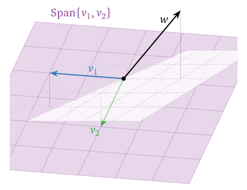
Figure \(\PageIndex{1}\)
It does not appear that \(w\) lies in \(\text{Span}\{v_1,v_2\},\) so the equation is inconsistent.

Let us check our geometric answer by solving the matrix equation using row reduction. We put the system into an augmented matrix and row reduce:
\[\left(\begin{array}{cc|c} 2&1&0 \\ -1&0&2 \\ 1&-1&2\end{array}\right) \quad\xrightarrow{\text{RREF}}\quad \left(\begin{array}{cc|c} 1&0&0 \\ 0&1&0 \\ 0&0&1\end{array}\right).\nonumber\]
The last equation is \(0=1\text{,}\) so the system is indeed inconsistent, and the matrix equation
\[\left(\begin{array}{cc}2&1\\-1&0\\1&-1\end{array}\right)x=\left(\begin{array}{c}0\\2\\2\end{array}\right)\nonumber\]
has no solution.
Let \(A=\left(\begin{array}{cc}2&1\\-1&0\\1&-1\end{array}\right)\). Does the equation \(Ax=\left(\begin{array}{c}1\\-1\\2\end{array}\right)\) have a solution?
Solution
First we answer the question geometrically. The columns of \(A\) are
\[\color{Red}{v_1=\left(\begin{array}{c}2\\-1\\1\end{array}\right)}\quad\color{black}{\text{and}}\quad\color{blue}{v_2 =\left(\begin{array}{c}1\\0\\-1\end{array}\right)},\nonumber\]
and the target vector (on the right-hand side of the equation) is \(\color{Green}{w=\left(\begin{array}{c}1\\-1\\2\end{array}\right)}\). The equation \(Ax=w\) is consistent if and only if \(w\) is contained in the span of the columns of \(A\). So we draw a picture:
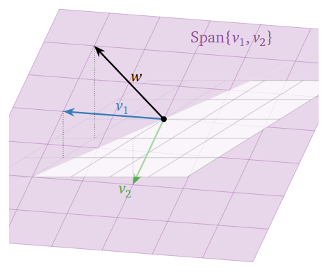
Figure \(\PageIndex{3}\)
It appears that \(w\) is indeed contained in the span of the columns of \(A\text{;}\) in fact, we can see
\[ w = v_1 - v_2 \implies x = \left(\begin{array}{c}1\\-1\end{array}\right). \nonumber \]
Let us check our geometric answer by solving the matrix equation using row reduction. We put the system into an augmented matrix and row reduce:
\[\left(\begin{array}{cc|c}2&1&1\\-1&0&-1\\1&-1&2\end{array}\right) \quad\xrightarrow{\text{RREF}}\quad \left(\begin{array}{cc|c} 1&0&1 \\ 0&1&-1 \\ 0&0&0\end{array}\right).\nonumber\]
This gives us \(x=1\) and \(y=-1\text{,}\) which is consistent with the picture:
\[1\left(\begin{array}{c}2\\-1\\1\end{array}\right)-1\left(\begin{array}{c}1\\0\\-1\end{array}\right)=\left(\begin{array}{c}1\\-1\\2\end{array}\right)\quad\text{or}\quad A\left(\begin{array}{c}1\\-1\end{array}\right)=\left(\begin{array}{c}1\\-1\\2\end{array}\right).\nonumber\]
When Solutions Always Exist.
Building on the Note \(\PageIndex{6}\): Spans and Consistency, we have the following criterion for when \(Ax=b\) is consistent for every choice of \(b\).
Let \(A\) be an \(m\times n\) (non-augmented) matrix. The following are equivalent:
- \(Ax=b\) has a solution for all \(b\) in \(\mathbb{R}^m\).
- The span of the columns of \(A\) is all of \(\mathbb{R}^m\).
- \(A\) has a pivot position, Definition 1.2.5 in Section 1.2, in every row.
- Proof
-
The equivalence of 1 and 2 is established by the Note \(\PageIndex{6}\): Spans and Consistency as applied to every \(b\) in \(\mathbb{R}^m\).
Now we show that 1 and 3 are equivalent. (Since we know 1 and 2 are equivalent, this implies 2 and 3 are equivalent as well.) If \(A\) has a pivot in every row, then its reduced row echelon form looks like this:
\[\left(\begin{array}{ccccc}1&0&\star &0&\star \\ 0&1&\star &0&\star \\ 0&0&0&1&\star \end{array}\right),\nonumber\]
and therefore \(\left(\begin{array}{c|c}A&b\end{array}\right)\) reduces to this:
\[\left(\begin{array}{ccccc|c} 1&0&\star &0&\star &\star \\ 0&1&\star &0&\star &\star \\ 0&0&0&1&\star &\star\end{array}\right).\nonumber\]
There is no \(b\) that makes it inconsistent, so there is always a solution. Conversely, if \(A\) does not have a pivot in each row, then its reduced row echelon form looks like this:
\[\left(\begin{array}{ccccc}1&0&\star &0&\star \\ 0&1&\star &0&\star \\ 0&0&0&0&0\end{array}\right),\nonumber\]
which can give rise to an inconsistent system after augmenting with \(b\text{:}\)
\[\left(\begin{array}{ccccc|c} 1&0&\star &0&\star &0 \\ 0&1&\star &0&\star &0 \\ 0&0&0&0&0&16\end{array}\right).\nonumber\]
Recall that equivalent means that, for any given matrix \(A\text{,}\) either all of the conditions of the above Theorem, \(\PageIndex{1}\), are true, or they are all false.
Be careful when reading the statement of the above Theorem, \(\PageIndex{1}\). The first two conditions look very much like this Note \(\PageIndex{6}\): Spans and Consistency, but they are logically quite different because of the quantifier “for all \(b\)”.
We will see in this Corollary 2.7.1 in Section 2.7 that the dimension of the span of the columns is equal to the number of pivots of \(A\). That is, the columns of \(A\) span a line if \(A\) has one pivot, they span a plane if \(A\) has two pivots, etc. The whole space \(\mathbb{R}^m\) has dimension \(m\text{,}\) so this generalizes the fact that the columns of \(A\) span \(\mathbb{R}^m\) when \(A\) has \(m\) pivots.